Upgraded Marketing Mix Modeling in Python

Marketing Analytics

Flashback

In my last article, I introduced you to the world of marketing mix modeling. If you have not read it so far, please do before you proceed.

Introduction to Marketing Mix Modeling in Python

There, we have created a linear regression model that is able to predict sales based on raw advertising spends in several advertising channels, such as TV, radio, and web banners. As a Machine Learning practitioner, such a model is already lovely on its own. Even better, it also makes business people happy because the model lets us calculate ROIs, allowing us to judge how well each channel performed.

However, our simple linear regression model from last time had some issues that we will resolve in this article. Let me paraphrase them for you:

The performance of our first model could be better.
Our first model behaves unrealistically. Increasing the spendings to infinity also increases the sales to infinity, which makes no sense because people can only spend a finite amount of money on our product.
Optimizing becomes trivial, useless, and unrealistic as well. We would now put all the money into the channel with the highest linear regression coefficient to maximize sales given a fixed budget.

Advertising

I created a small library where I implemented the ideas from the rest of the article and even more. install it via pip install mamimo and check out how to use it here:

A Small Python Library For Marketing Mix Modeling: MaMiMo

Fixing the Problems

To circumvent these problems, we can do some clever feature engineering that allows us to incorporate some Marketing domain knowledge into the model. Do not worry; marketing experience is not required to understand these concepts – they come pretty naturally. The following techniques will improve performance and make the model more realistic.

Advertising Adstock

This feature engineering that we will do is a crucial component called advertising adstock, a term coined by Simon Broadbent [1]. It is a fancy word that encapsulates two simple concepts:

We assume that the more money you spend on advertising, the higher your sales get. However, the increase gets weaker the more we spend. For example, increasing the TV spends from 0 € to 100,000 € increases our sales a lot, but increasing it from 100,000,000 € to 100,100,000 € does not do that much anymore. This is called a saturation effect or the __ effect of diminishing returns.
If you spend money on advertising week T, often people will not immediately buy your product, but a few (let us say x) weeks later. This is because the product might be expensive, and people want to think about it carefully or compare it to similar products from other companies. Whatever the reason might be, the sale in week T + x is partially caused by the advertising you played in week T, so it should also get some credits. This is called the carryover or lagged effect.

Both facts are pretty easy to understand, and business people dig them.

Our new model is still linear, but with adstock features instead of raw spendings as input. This makes the model much stronger while keeping it interpretable.

Building Saturation and Carryover Effects in scikit-learn

Unfortunately for us, scikit-learn does not contain these transformations because they are not of cross-industry interest. But since both transformations are not complicated, it is an excellent opportunity to practice writing scikit-learn compatible estimators.

If this is your first time doing that, you can check out my other article just about that topic. The article is about regressors rather than transformers, but the approach is similar.

Build your own custom scikit-learn Regression

So, let’s start with the easier one: the saturation effect.

Creating a Saturation Effect

We want to create a transformation (=mathematical function) with the following properties:

If the spendings are 0, the saturated spendings are also 0.
The transformation is monotonically increasing, i.e., the higher the input spendings, the higher the saturated output spendings.
The saturated values do not grow to infinity. Instead, they are upper bounded by some number, let us say 1.

In short, we want something like this:

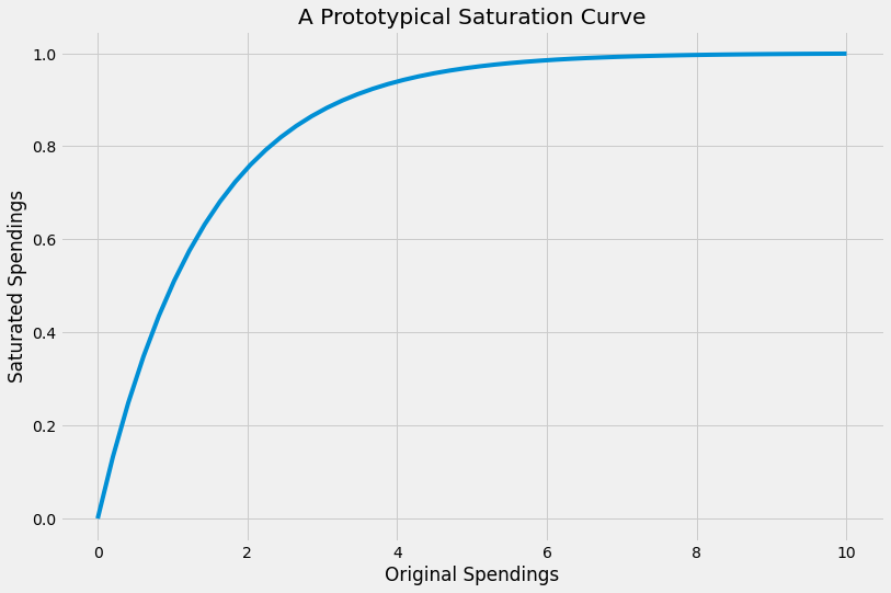
There are many ways to get functions like this. In the picture you see the function 1-exp(-0.7x), for example. So let us use this function template and generalize it to 1-exp(-ax) for some a > 0. a is a hyperparameter that we can tune afterward because usually, we do not know the shape of the saturation function.

Note: There are many more standard saturations functions, such as the Adbudg and Hill functions, but let us stick with the exponential function **** for simplicity.

A nice side-effect: We are able to output the saturation curves in the end, so we know if it makes sense to spend more money or if the channel is saturated already. From the picture above, investing more than eight seems useless.

So, let’s code this. In fact, it is just this simple little class:

class ExponentialSaturation:
    def __init__(self, a=1.):
        self.a = a

    def transform(self, X):
        return 1 - np.exp(-self.a*X)

However, we will add some sanity checks for the inputs to make it scikit-learn compliant. This bloats up the code a bit, but this price is comparatively low.

from sklearn.base import BaseEstimator, TransformerMixin
from sklearn.utils.validation import check_is_fitted, check_array

class ExponentialSaturation(BaseEstimator, TransformerMixin):
    def __init__(self, a=1.):
        self.a = a

    def fit(self, X, y=None):
        X = check_array(X)
        self._check_n_features(X, reset=True) # from BaseEstimator
        return self

    def transform(self, X):
        check_is_fitted(self)
        X = check_array(X)
        self._check_n_features(X, reset=False) # from BaseEstimator
        return 1 - np.exp(-self.a*X)

It still needs improvement because we should also implement a check for a being larger than zero, but this is something you can easily do on your own. With the ExponentialSaturation transformer, we can do the following:

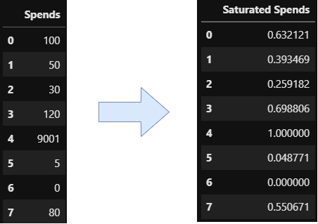
This one was not too bad, right? Let us now move on to the next effect.

Creating a Carryover Effect

This one is slightly more tricky. Let me use an example to show you what we want to achieve. We are given a series of spendings over time, such as

(16, 0, 0, 0, 0, 4, 8, 0, 0, 0),

meaning that we spent 16 in the first week, nothing from week 2 to 5, 4 in week 6, etc.

We now want that spendings in one week to get partially carried over to the following weeks in an exponential fashion. This means: In week 1 there is a spend of 16. Then we carry over 50%, meaning

0.5 * 16 = 8 to week 2,
0.5² * 16 = 4 to week 3,
0.5³ * 16 = 2 to week 4,
…

This introduces two hyperparameters: the strength (how much gets carried over?) and the length (how long does it get carried over?) of the carryover effect. If we use a strength of 50% and a length of 2, the spending sequence from above becomes

(16, 8, 4, 0, 0, 4, 10, 5, 2, 0).

I believe that you can write some loops to implement this behavior; a nice and fast way is using convolutions, though. I will not explain it in detail, so just take the code as a present.

from scipy.signal import convolve2d
import numpy as np

class ExponentialCarryover(BaseEstimator, TransformerMixin):
    def __init__(self, strength=0.5, length=1):
        self.strength = strength
        self.length = length

    def fit(self, X, y=None):
        X = check_array(X)
        self._check_n_features(X, reset=True)
        self.sliding_window_ = (
            self.strength ** np.arange(self.length + 1)
        ).reshape(-1, 1)
        return self

    def transform(self, X: np.ndarray):
        check_is_fitted(self)
        X = check_array(X)
        self._check_n_features(X, reset=False)
        convolution = convolve2d(X, self.sliding_window_)
        if self.length > 0:
            convolution = convolution[: -self.length]
        return convolution

You can see that the class takes the strength and length. During the fit, it creates a sliding window that gets used by the convolve2d function, doing magically just what we want. If you know convolutional layers from CNNs, this is exactly what happens here. Graphically, it does the following:

Note: There are many more ways to create a carryover as well. The decay does not have to be exponential. And maybe the peak of the advertising effect is not reached on the day the money was spent, but always the next week. You can express all of these variations by changing the sliding window accordingly.

Let us combine both saturation and carryover effects to create a more realistic marketing mix model.

The Final Model

We will use different saturations and carryovers for each channel. This makes sense because a TV ad usually sticks longer in your head than a banner you see online, for example. From a high-level perspective, the model will look like this:

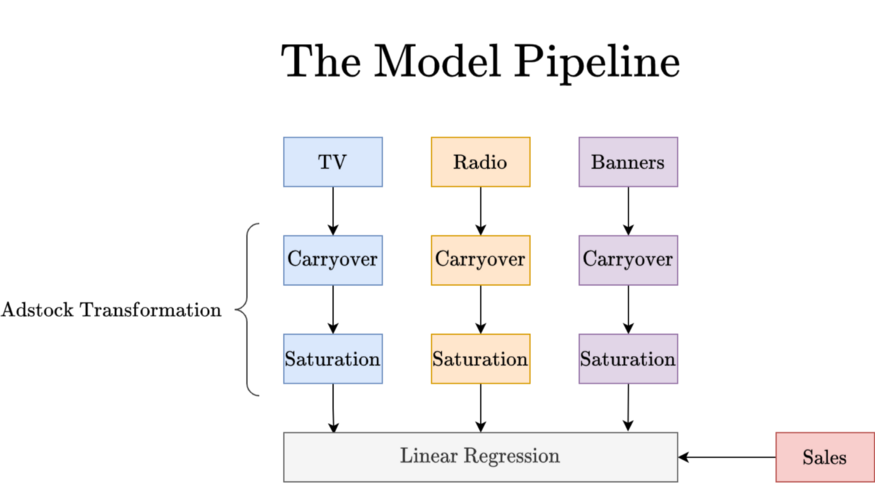
Note that the blue pipeline is just a function of the TV spendings, the orange one of radio spendings, and the purple one of banner spendings. We can efficiently implement this in scikit-learn using the ColumnTransformer and Pipeline classes. The ColumnTransformer allows us to use a different transformation for each ad channel while the Pipeline enables us to chain operations for a single channel. Take a second to understand the following snippet:

from sklearn.compose import ColumnTransformer
from sklearn.pipeline import Pipeline
from sklearn.linear_model import LinearRegression

adstock = ColumnTransformer(
    [
     #### TV block ####
     ('tv_pipe', Pipeline([
                           ('carryover', ExponentialCarryover()),
                           ('saturation', ExponentialSaturation())
     ]), ['TV']),
     ('radio_pipe', Pipeline([
                           ('carryover', ExponentialCarryover()),
                           ('saturation', ExponentialSaturation())
     ]), ['Radio']),
     ('banners_pipe', Pipeline([
                           ('carryover', ExponentialCarryover()),
                           ('saturation', ExponentialSaturation())
     ]), ['Banners']),
    ],
    remainder='passthrough'
)

model = Pipeline([
                  ('adstock', adstock),
                  ('regression', LinearRegression())
])

The most difficult part is the ColumnTransformer. Let me explain how you can read the marked TV block. **** It just says:

Apply the pipeline to the column ‘TV’ and name this part ‘tv_pipe’. The pipeline is just the adstock transformation.

Nothing more is going on there. And in the end, we use this big preprocessing step and add a simple LinearRegression to the end to have an actual regressor. So, let us load the data again and do some training.

import pandas as pd
from sklearn.model_selection import cross_val_score, TimeSeriesSplit

data = pd.read_csv(
    'https://raw.githubusercontent.com/Garve/datasets/4576d323bf2b66c906d5130d686245ad205505cf/mmm.csv',
    parse_dates=['Date'],
    index_col='Date'
)

X = data.drop(columns=['Sales'])
y = data['Sales']

model.fit(X, y)

print(cross_val_score(model, X, y, cv=TimeSeriesSplit()).mean())

# Output: ~0.55

Note: We do not use the standard k_-fold cross-validation here because we are dealing with time series data. TimeSeriesSplit is a more reasonable thing to do, and you can read more about it here._

It works! However, the model is still quite bad, with a cross-validated _r_² of about 0.55, while the old, simpler model had one of 0.72. This is because we used the default and hence non-optimal parameters for each channel, namely a = 1 for saturation, a carryover strength of 0.5, and a length of 2.

So, let us tune all the adstock parameters!

Hyperparameter Tuning

I will use Optuna, an advanced library for optimization tasks. Among many other things, it offers a scikit-learn-compatible OptunaSearchCV class that you can see as a drop-in replacement of scikit-learn’s [GridSearchCV](https://scikit-learn.org/stable/modules/generated/sklearn.model_selection.GridSearchCV.html) and [RandomizedSearchCV](https://scikit-learn.org/stable/modules/generated/sklearn.model_selection.RandomizedSearchCV.html) .

In a nutshell, OptunaSearchCV is a much smarter version of RandomizedSearchCV . While RandomizedSearchCV walks around randomly only, OptunaSearchCV walks around randomly at first but then checks hyperparameter combinations that look most promising.

Check out the code that is quite close to what you are used to writing in scikit-learn:

from optuna.integration import OptunaSearchCV
from optuna.distributions import FloatDistribution, IntDistribution

tuned_model = OptunaSearchCV(
    estimator=model,
    param_distributions={
        'adstock__tv_pipe__carryover__strength': FloatDistribution(0, 1),
        'adstock__tv_pipe__carryover__length': IntDistribution(0, 6),
        'adstock__tv_pipe__saturation__a': FloatDistribution(0, 0.01),
        'adstock__radio_pipe__carryover__strength': FloatDistribution(0, 1),
        'adstock__radio_pipe__carryover__length': IntDistribution(0, 6),
        'adstock__radio_pipe__saturation__a': FloatDistribution(0, 0.01),
        'adstock__banners_pipe__carryover__strength': FloatDistribution(0, 1),
        'adstock__banners_pipe__carryover__length': IntDistribution(0, 6),
        'adstock__banners_pipe__saturation__a': FloatDistribution(0, 0.01),
    },
    n_trials=1000,
    cv=TimeSeriesSplit(),
    random_state=0
)

You tell Optuna to optimize model . It does so by using all parameters you specify in param_distributions . Because our model is quite nested, i.e., there are pipelines in a column transformer that itself is in a pipeline again, we have to specify precisely which hyperparameter we want to tune. This is done via strings such as adstock__tv_pipe__carryover__strength , where two underscores separate different levels of the complete model. You find the words adstock , tv_pipe , carryover all in the model specification, while strength is a parameter of the ExponentialCarryover transformer.

Then, you find some distributions. FloatDistribution(0, 1) means that it should look for float parameters between 0 and 1. By the same logic, IntDistribution(0, 6) searches for integer values between 0 and 6 (not 5!). Thus we tell the model only to consider carryover length less or equal to six weeks, which is just a choice we make.

We try n_trials=1000 different combinations of parameters and evaluate using a TimeSeriesSplit again. Keep the results reproducible by setting random_state=0 . Done! This should be enough to understand the code.

Performance Check

Let us check the performance using this optimized model named tuned_model . Be careful – this takes a long time. You can reduce the n_trials to 100 to get a worse solution much faster.

print(cross_val_score(tuned_model, X, y, cv=TimeSeriesSplit()))

# Output: array([0.847353, 0.920507, 0.708728, 0.943805, 0.908159])

Update: Currently, I get an error when executing the Optuna version. Probably the library changed a lot in the meantime. If you can’t get it to work, use this version instead of the Optuna one:

from sklearn.model_selection import RandomizedSearchCV
from scipy.stats import uniform, randint

tuned_model = RandomizedSearchCV(
    estimator=model,
    param_distributions={
        'adstock__tv_pipe__carryover__strength': uniform(0, 1),
        'adstock__tv_pipe__carryover__length': randint(0, 6),
        'adstock__tv_pipe__saturation__a': uniform(0, 0.01),
        'adstock__radio_pipe__carryover__strength': uniform(0, 1),
        'adstock__radio_pipe__carryover__length': randint(0, 6),
        'adstock__radio_pipe__saturation__a': uniform(0, 0.01),
        'adstock__banners_pipe__carryover__strength': uniform(0, 1),
        'adstock__banners_pipe__carryover__length': randint(0, 6),
        'adstock__banners_pipe__saturation__a': uniform(0, 0.01),
    },
    n_iter=1000,
    cv=TimeSeriesSplit(),
    random_state=0
)

The mean cross-validated _r_² is 0.87, which is a considerable improvement compared to the unoptimized model (0.55) and our old plain linear model from the last article (0.72). Let us now refit the model and see what it has learned.

tuned_model.fit(X, y)

The optimal hyperparameters are the following:

print(tuned_model.best_params_)
print(tuned_model.best_estimator_.named_steps['regression'].coef_)
print(tuned_model.best_estimator_.named_steps['regression'].intercept_)

# Output:
# Hyperparameters = {
# 'adstock__tv_pipe__carryover__strength': 0.5248878517291329
# 'adstock__tv_pipe__carryover__length': 4
# 'adstock__tv_pipe__saturation__a': 1.4649722346562529e-05
# 'adstock__radio_pipe__carryover__strength': 0.45523455448406197
# 'adstock__radio_pipe__carryover__length': 0
# 'adstock__radio_pipe__saturation__a': 0.0001974038926379962
# 'adstock__banners_pipe__carryover__strength': 0.3340342963936898
# 'adstock__banners_pipe__carryover__length': 0
# 'adstock__banners_pipe__saturation__a': 0.007256873558015173
# }
#
# Coefficients = [27926.6810003   4114.46117033  2537.18883927]
# Intercept = 5348.966158957056

Using the Model for New Data

In case you want to create forecasts for a new spending table, you can proceed like this:

X_new = pd.DataFrame({
    'TV': [10000, 0, 0],
    'Radio': [0, 3000, 0],
    'Banners': [1000, 1000, 1000]
})

tuned_model.predict(X_new)

Note that the prediction always starts out with an adstock of zero, i.e. the model does not know about any carryovers from the past unless you put it into your prediction data frame. For example, if you want to know the sales in week w, and you feed the model only the spendings of week w, it will not consider carryovers from the weeks w-1, w-2, … before. You have to include the weeks before as well if you want the model to build up an adstock, even if you are only interested in the prediction for the last observation.

You can even extend the training data with more features that are not spendings, so-called control variables. If you do not specify any preprocessing in the ColumnTransformer object, the raw values will directly get passed to the LinearRegression and be considered for training and predictions.

Interpreting the Model

Using the data from above, we can create some pretty pictures that help us get insights from the model.

Saturation Effects

If we plug in the values for the saturation transformers, we get the following:

We can see that the model thinks that the channel TV is still quite undersaturated – spending more here might benefit sales. Note that our maximum TV spending was about 15000.
Radio looks more saturated, but increasing the spendings here still seems reasonable. The maximum spending in this channel was about 7700.
The banners look oversaturated. The maximum spending here was about 2500, with a function value of nearly 1 already. Higher spendings do not seem to accomplish much.

Carryover Effects

If we plug in the values for the carryover transformers, we get the following:

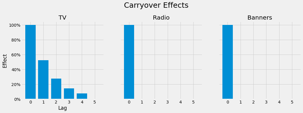
It seems that TV advertisings still affect sales four weeks later after the initial spending. This is much longer than the effect of radio and web banner spendings that quickly wears off in the same week.

Channel Contributions

As in the last article, we can calculate the contributions of each channel to the sales for each day. The code is slightly more complex than before because the model got more complicated as well. Anyway, here is a working version:

adstock_data = pd.DataFrame(
    tuned_model.best_estimator_.named_steps['adstock'].transform(X),
    columns=X.columns,
    index=X.index
)

weights = pd.Series(
    tuned_model.best_estimator_.named_steps['regression'].coef_,
    index=X.columns
)

base = tuned_model.best_estimator_.named_steps['regression'].intercept_

unadj_contributions = adstock_data.mul(weights).assign(Base=base)
adj_contributions = (unadj_contributions
                     .div(unadj_contributions.sum(axis=1), axis=0)
                     .mul(y, axis=0)
                    )

ax = (adj_contributions[['Base', 'Banners', 'Radio', 'TV']]
      .plot.area(
          figsize=(16, 10),
          linewidth=1,
          title='Predicted Sales and Breakdown',
          ylabel='Sales',
          xlabel='Date'
      )
     )

handles, labels = ax.get_legend_handles_labels()
ax.legend(
    handles[::-1], labels[::-1],
    title='Channels', loc="center left",
    bbox_to_anchor=(1.01, 0.5)
)

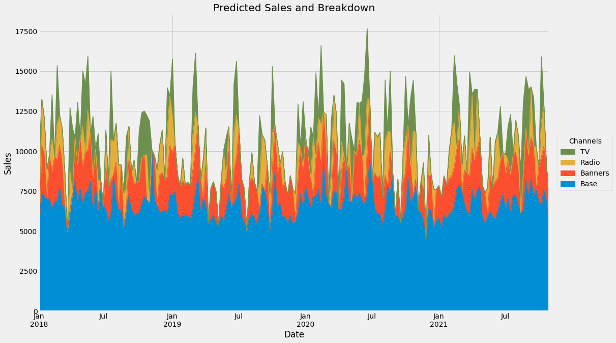
The output:

Compared to the old picture, the baseline is not so wiggly anymore because the model can explain the sales better with the given channel spendings. Here is the old one:

The old model. Image by the author. — The **old** model. Image by the author.

Summary and Outlook

In this article, we have taken our old and simple linear model and improved it by not relying on the raw channel spendings but on adstocks. The adstocks are transformed spendings that reflect the real world more realistically by introducing saturation and carryover effects.

We even did a concise implementation of both concepts that can be used within the scikit-learn ecosystem in a plug-and-play manner.

The last thing we did was tune the model and then take a look at what it has learned. We got some interesting insights in the form of pictures that people can easily understand, making this model both accurate and interpretable.

However, there are still some loose ends:

We have talked about optimizing spendings and how this was not possible with the old model. Well, with the new one it is, but I will not go into detail here. In short, treat our tuned_model as a black-box function and optimize it with a program of your choice, for example, Optuna or scipy.optimize.minimize. Add some budget constraints to the optimization, such as the sum of spendings should be less than 1,000,000.
Feeding non-spending data into the model might improve it even more. Take the day of the week, the month, or the price of the product we want to sell, for example. Especially the price is an essential driver for sales: A regular iPhone offered for 10000 € would not generate many sales, while one for 100 € would be out of stock in a blink of an eye. Time features like the month can be interesting for seasonal products like fans or hot chocolate. Or special days like Christmas. Gather your thoughts, and make sure to add everything that can influence the sales!