
Linear regression is one of the most basic Machine Learning models out there, yet its application is everywhere: from predicting housing prices to predicting movie ratings. Even when you’re taking a cab to go to work, you have a linear regression problem to deal with.
Simply put, linear regression relates to the linear relationship between the predicted value and feature value. The mathematical equation of linear regression is as follows:

where Y is the predicted value, θ₀ is the bias parameter, θ₁ is the parameter value, and x is the feature value.
To illustrate what these parameters mean, consider you’re taking a taxi to go to work. Soon after you enter the taxi, the taxi fare wouldn’t be starting from 0. Instead, it starts from some values, let’s say $5. This $5 represents the bias term in the Regression equation (θ₀). The predicted value Y would be the price that you should pay, the feature value x would be the travel distance, and θ₁ is the slope on how much more do you need to pay as the travel distance is increased.
Let’s generate a random linear-look data between taxi fare and travel distance to visualize the illustration above.
import numpy as npnp.random.seed(1)
x = 2 * np.random.rand(100,1)
y = 4+ 2 * x + np.random.rand(100,1)
There is a linear trend there between taxi fare and travel distance. Hence we can relate taxi fare and travel distance as a linear function:

Now the problem is how do we obtain the optimum value of θ₀ and θ₁ such that our linear regression model perform best? We can use Scikit-learn for that.
Building Linear Regression Model with Scikit-learn
If you have a linear regression problem to solve like in the study case above, the easiest way to find the optimum value of θ₀ and _θ₁_is by calling LinearRegression function from Scikit-learn library. The problem can be solved in just four lines of code as follows:
from sklearn.linear_model import LinearRegressionlm = LinearRegression()#train the model
lm.fit(x,y)print(lm.intercept_, lm.coef_)## Output: [4.49781698] [[1.98664487]]which gives us the relationship between taxi fare and travel distance as follows:

By having this relationship, now you can plug the travel distance between your position and your destination and now you can predict how much money you should pay for your taxi fare.
Linear Regression More than Just a Black Box
It is amazing what Machine Learning libraries can do to make our life easier to solve different problems. With just four lines of code, you optimized a linear regression model already without knowing anything under the hood.
While these Machine Learning libraries are amazing, but they certainly hide some implementation details for you, i.e we have treated linear regression problems as a black box.
Wouldn’t it be awesome to know what is under the hood and how Scikit-learn come up with the solution _taxi_fares = 4.49 + 1.98*traveldistance? How do they know that 4.49 is the optimum value for the bias term and 1.98 is the optimum value for the slope?
If we know what happens under the hood, we will have a deep understanding of the appropriate model to use in any given problem and we can debug the errors more effectively. Plus, having a good understanding of how regression problem works would be a good foundation for us to understand the mathematics and intuition behind neural networks algorithm.
To find the optimum model for linear regression problems, normally there are two ways:
- Using iterative optimization approach called Gradient Descent.
- Using ‘closed-form’ equation called Normal Equation.
Gradient Descent for Linear Regression
In a nutshell, Gradient Descent algorithm finds the optimum solution for a linear regression problem by tweaking model parameters θ (the bias term and the slope) to minimize the error or cost function with respect to training data iteratively.
Let’s visualize how Gradient Descent works to make it clearer.

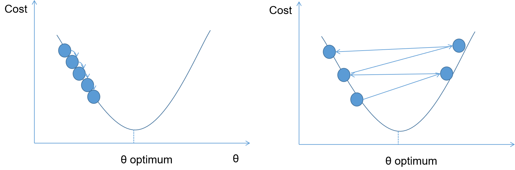
Gradient Descent starts by randomly initializing an initial value of parameter value θ. This θ value then will be tweaked in every iteration such that the error or cost function is minimized. Once the Gradient Descent algorithm finds θ minimum, the cost function wouldn’t get smaller any further. This means that the algorithm has converged.
It is important to note that not all of the cost functions have a perfectly nice bowl shaped like in the image above. Most of the times, the cost function has all sorts of irregular shapes and plateaus like this:

The shape irregularity of the cost function makes it difficult for Gradient Descent algorithm to converge, as there is a huge chance that the algorithm will be stuck at the local optima and not finding the global optimum.
Fortunately, the cost function in a linear regression problem is always convex, meaning that there will be no local optima, just one global optimum solution. Thus, no matter how and where you initialize your initial value, it can ‘almost’ be guaranteed that the Gradient Descent algorithm will end up in the global minimum solution.
But the question is, why is it ‘almost’ be guaranteed that Gradient Descent will end up in the global minimum if there are no local optima?
Because there is one important parameter in Gradient Descent that you need to define in advance, which is the learning rate.
The learning rate determines how big is the step the algorithm should take in each iteration. If the learning rate is too small, there is a good chance that the global minimum wouldn’t be reached at the end of iterations. If the learning rate is too high, the algorithm will jump around the valley at each iteration and the algorithm will diverge.
Implementation of Gradient Descent
After all of the explanation about Gradient Descent, let’s implement it with a code using the study case taxi fare vs travel distance.
For a linear regression problem, the cost function of Gradient Descent algorithm that we should minimize is the mean squared error (MSE).

where:

In the mathematical notation above, J is the cost function, m is the number of observations or data, hθ is the predicted value from linear regression, θ₀ is the bias term, θ₁ is the slope, x is the feature value and y is the actual predicted value. We can implement above equations in a code:
def computeCostFunction(x, y, theta, num_observations):

    linear_function= np.matmul(x,theta)
    error = np.subtract(linear_function,y)
    error_squared = error.transpose()**2
    cost_function = (0.5/num_observations)*(np.sum(error_squared))

    return cost_function
The next important step is to compute the gradient of the cost function for each model parameter θⱼ. The intuition behind this gradient is how much the cost function will change if you tweak the value of parameter θⱼ.
For mean squared error, there is a closed form solution for its partial derivative. So, it is not a problem if you’re not an expert in Calculus.

Once you know the gradient of each parameter θⱼ, now you can update each parameter θⱼ for one iteration. This is where the learning rate α plays a role in a Gradient Descent algorithm.

Finally, we can implement the above equations in a code:
intercept_x = np.ones((len(x),1)) #add bias term
x = np.column_stack((intercept_x,x))
alpha = 0.05 #learning rate
iterations = 25000
theta = np.random.randn(2,1) #random initialization of parameters
num_observations = 1000def gradientDescent(x, y, theta, alpha, num_observations, iterations):
cost_history = np.zeros((iterations,1))
for i in range (iterations):
linear_function= np.matmul(x,theta)
error = np.subtract(linear_function,y) gradient = np.matmul(x.transpose(),error)
theta = theta - (alpha * (1/num_observations) * gradient)
cost_history[i] = computeCostFunction(x, y, theta, num_observations)
return theta, cost_historytheta, cost_history = gradientDescent(x, y, theta, alpha, num_observations, iterations)print(theta)#Output: array([[4.49781697],[1.98664487]])The output from Gradient Descent looks the same from the one obtained with Scikit-learn. The difference is that you now know what’s under the hood.
There is one more straightforward approach to find the optimum solution for your linear regression problem, which is the Normal Equation.
The Normal Equation
In linear regression, the Normal Equation is a closed-form solution to find the optimum value for the parameters. With this approach, there is no iterative approach, no partial derivatives, and no parameter updates. Once you compute the Normal Equation, then you’re done and you get the optimum solution for your linear regression model.

In the equation above, θ is the optimum value of regression parameters, x is the feature and Y is the predicted value. We can implement the equation above in a code:
def normalEquation(x, y):

    x_transpose = x.transpose()
    x = np.matmul(x_transpose, x)
    x_inverse = np.linalg.inv(x)
    x_final = np.matmul(x_inverse,x_transpose)

    theta = np.matmul(x_final,y)

    return theta
theta = normalEquation(x, y)print(theta)#Output: array([[4.49781698],[1.98664487]])
And again, the result matched with the one we got from Scikit-learn library and Gradient Descent optimization. Now you might ask a question: if the Normal Equation is very straightforward, then why shouldn’t we use it instead of Gradient Descent? Let’s discuss that.
Normal Equation or Gradient Descent?
Both Normal Equation and Gradient Descent have their own advantages and disadvantages when it comes to solving a linear regression problem.
With Normal Equation, the solution for a linear regression problem can be solved directly, with no need for initializing initial parameter value θⱼ and no need to compute the partial derivatives. All can be done using matrix vectorization. This makes everything fast even when the number of observations or training data is huge. Moreover, you don’t need to normalize each parameter for Normal Equation to come up with an optimum solution.
The major disadvantage of using Normal Equation is its computational complexity. This is because we need to invert the matrix with this method. If you have a multiple linear regression problem with a huge selection of features, the computation cost of Normal Equation will be very expensive.
With Gradient Descent, the computational complexity wouldn’t be a problem if you have a huge selection of features in a multiple linear regression problem.
However, Gradient Descent is becoming much slower if you have a huge amount of observations or training data. This is because at each iteration, Gradient Descent uses all of the training data to compute the cost function.
Moreover, you always need to normalize or scale each of your features to make Gradient Descent converge faster. Below is the illustration if you normalize the features vs if you forget to normalize your features.
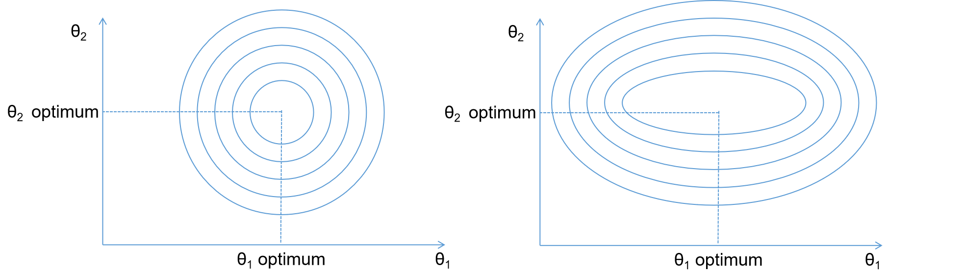
If you normalize your features, the cost function in linear regression forms a perfect bowl shape which makes it faster for the algorithm to converge. Meanwhile, the elongated bowl shape will be formed if you forget to normalize the features or they don’t share the same scale. The algorithm will eventually still end-up in the global minimum solution, but it will take a longer time to converge.
Now you know the advantages and disadvantages of using Normal Equation and Gradient Descent algorithm. As a takeaway, below is the table summarizing the performance of both algorithms.

How to Improve the Performance of Gradient Descent?
The major disadvantage of Gradient Descent is that it uses the whole training data to compute the cost function at every iteration. This will be problematic if we have a huge number of observations or training data. To solve the problem, normally Stochastic Gradient Descent (SGD) or Mini-Batch Gradient Descent is applied instead.
In SGD algorithm, instead of using the whole training example, this algorithm will pick a random instance in the training example at every step. Then, the gradient will be computed based on this random instance. This makes the computation time faster and less expensive, since only one instance needs to be in the memory at each step.
In Mini-Batch Gradient Descent, instead of using the whole training example like Gradient Descent or using a random instance like SGD, the gradient will be computed based on a small subset of random instances called mini-batches. Dividing the whole training data into several small mini-batches makes the matrix operations and computation process faster.
For a simple or multiple linear regression problem, normally using Gradient Descent is enough. However, for more complex applications such as neural networks algorithm, Mini-Batch Gradient Descent will be preferred.


