The conundrum of the data scientist: we’ve cleaned the data, made the modeling assumptions and eagerly booted up sklearn; all that stands between us and Kaggle competition glory are these pesky hyperparameters. How do we choose them?
Model performance often boils down to three key ingredients: the data, model appropriateness and choice of hyperparameters. We can think of the data and model class as ingredients in the greatest conceivable blueberry muffin recipe, but even these won’t salvage the product of a baker who sets them in a 300°C oven for three hours. How do we help him find these optimal settings?
Hyperparameter Optimization
The art of optimizing model hyperparameters is termed, you guessed it, hyperparameter optimization. During this stage of modeling, we posit the question: what choice of model settings gives the best performance on my validation dataset?
Note: model hyperparameters should be distinguished from model parameters. Model parameters are learned from the data whilst hyperparameters are chosen by us, the data scientists. For example, when fitting a linear model of the form:

we are learning β from our data y and X. If X contains many features with some underlying correlation structure, we might want to use something like L1, L2 or elasticNet regularization to reduce overfitting.
Hyperparameter optimization helps us answer questions like: "what regularization method should I choose?" and "what value for the regularizing parameter should I set?". We can tune other models like random forest regressor by asking "how many trees do I need?" and "what should the maximum tree depth be?".
Grid Search
The simplest way to do this would be to fit our model using every hyperparameter combination and settle on that providing the best performance on a hold-out validation set. This method is called Grid Search optimization because we can imagine each combination as a point on a grid spanned by the values each hyperparameter can take.

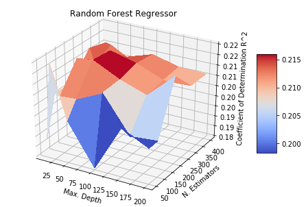
Above are two model classes tuned over a toy dataset with 100 features and 1000 samples. In this grid-search, each pair of hyperparameters is used to train a new model with validation performance evaluated over a hold-out dataset. While this is relatively feasible in the Elastic Net model (Fig 1. Left), it can be extremely computationally expensive in the case of a non-parametric model class like Random Forest Regression (Fig 1. Right).
Grid search is a deterministic approach to Hyperparameter Tuning: we consider each hyperparameter configuration independently. A key observation of the surfaces in Fig 1. are that they are continuous and well-behaved (if we know any point on the surface with certainty, we can take a decent guess at the values right next to it). So if we take a probabilistic approach instead, we can approximate the surfaces in Fig 1. using far fewer numbers of trained models. This is where Bayesian Optimization is incredibly useful.
Bayesian Optimization
Bayes rule lets us ask the following question: I have some prior belief about how my error surface will look like, I have a model class and data that I can use to gather more evidence, how can I update my error surface using newly gathered evidence to give me a posterior estimate of the optimal hyperparameter?
To begin, we need a flexible, scalable and well-behaved model to approximate the error surface of my regression model w.r.t our hyperparameters. In Bayesian Optimization this is called the surrogate model. Suppose we are tuning Lambda hyperparameter of a Ridge regression model, which takes values in [0,1] in python’s sklearn implementation.
We hypothesize that our validation error is a function of this hyperparameter but aren’t sure what form this function takes. Since we don’t have any evidence yet, we can start by assuming an uninformative structure where each error value is independently drawn from a standard normal distribution with mean 0 and a standard deviation of 1. This is plotted over the Lambda domain in Fig 2. below.

You can imagine an infinite number of individual normal distributions assembled along the x-axis, with the shaded area representing +/-1 standard deviations away from the mean centered at 0. We stated earlier that our confidence regarding the value of a proposed point should increase when the points near to it are known; we need to encode this dependency in a covariance structure.
This is where kernel functions are especially useful, they measure the similarity between any two given points and can be used to set up a prior distribution over all possible covariance matrices. Similar L1-Ratio values are more likely to have similar distributions for the model error than distant values, and this is encoded in our choice of kernel function. The best thing about this is we can use it to set up prior distributions over functions. This construction has a special name: the Gaussian Process (GP) prior. An in-depth overview of GPs, including different types of kernel functions and their applications to Bayesian Optimization can be found here.
We will be using the Matern kernel as a prior for our surrogate function’s covariance matrix. Sampling values from our prior gives us a distribution of lines:

To update our prior, we can start with a random sample of Lambda and use it to update the surrogate function. Fitting a Ridge Regression model on the same toy dataset as before, we can compute the coefficient of determination at Lambda= 0.1; we see that the uncertainty around points adjacent to it shrinks considerably:

Ideally, we would like our next sample of Lambda to be one with a higher expected value for the coefficient of determination than our current sample. This is can be approached using an acquisition function function like Expected Improvement (EI). We can calculate this directly from our surrogate model and use it to propose the next point to evaluate.
We can iterate between evaluating, sampling, evaluating, sampling as long as we’d like; the modeler decides the trade-off between accuracy and computational load. Below are plots for a further four rounds of updates:


After only five rounds of Bayesian updates, we see that our surrogate function is taking a distinctive shape. The acquisition function is guiding our optimization away from higher values of Lambda which over-regularize the model.
To conclude: Bayesian Optimization using Gaussian Processes priors is an extremely useful tool for tuning model hyperparameters whilst minimizing overall computational overhead. For those interested in reading more, I would definitely recommend Peter Frazier‘s review on the area. An excellent python resource has been developed by Thomas Huijskens for Bayesian Optimization using Expected Improvement.
May the Bayesian force be with you and all your Kaggling endeavours.


