
Feel free to reuse images in any context without attribution (no rights reserved).
Motivation & Definition
Let’s start off with a motivating problem: tomography. Bonus, we’ll meet our eponymous Johann Radon.
Tomographic reconstruction is a type of multidimensional inverse problem where the challenge is to yield an estimate of a specific system from a finite number of projections. The mathematical basis for tomographic imaging was laid down by Johann Radon. Wikipedia
Under what real-world circumstances can we easily acquire projections without having easy access to the full volume? Surprisingly often! Let’s consider the case of brain imaging.
If we want to acquire a 3D volumetric image of a brain, we can relatively easily get integrated 2D slices. Think of an x-ray! We can pass energy through the volume and see how much of that energy makes it through. Each of these 2D x-ray images represents line integrals through the 3D volume. We can acquire lots of x-ray images at different geometries about the skull, e.g., from the left side, from the front, from the right side, and all the angles in between.
How, though, can we approximately reconstruct the underlying 3D volume given a set of 2D images acquired at arbitrary collection geometries?
If a function represents an unknown density, then the Radon transform represents the projection data obtained as the output of a tomographic scan. Hence the inverse of the Radon transform can be used to reconstruct the original density from the projection data […] Wikipedia
Let’s take a look at how the Radon transform (and its inverse) help us solve this exact problem!
Why should these particulars matter to the medical data scientist? Easy! An understanding of imaging methodology is critical to reasoning about the artifacts, limitations, and appropriate processing approaches for computer vision solutions.
Mechanics of the Radon Transform
For ease of visualization, let’s simplify our 3D brain with 2D integrated slices and instead consider a 2D image with 1D integrated slices. The logic is the same! This just makes our introduction less daunting.
Let’s get the fundamental observation out of the way! The Fourier slice theorem tell us…
If we take (n-1)-dimensional line integrals (like column sums) through an n-dimensional volume (like a 2D image), the (n-1)-dimensional Fourier transform of these integrals recover original n-dimensional Fourier values.
It will take a minute to unpack this! Let’s make it concrete: if I rotate a 2D image, sum the columns, and calculate the 1D FFT of these columns sums, I have recovered values from the 2D FFT of the original image. So, __ we can take advantage of the Fourier transform to implement the Radon transform!
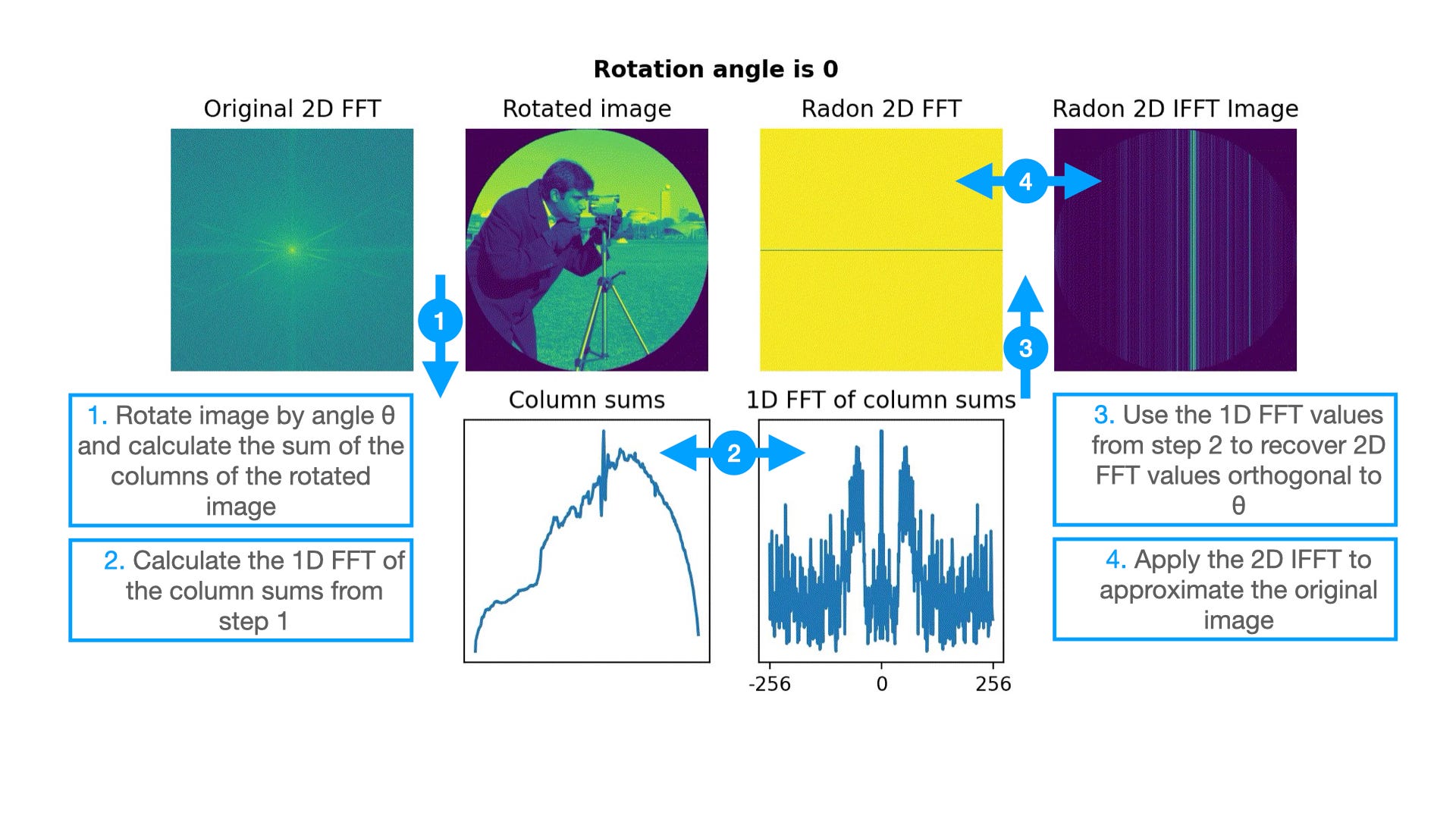
In Figure 1, the principle is shown for an image without rotation applied. We are just summing the columns of the original picture. If we take the 1D FFT of these column sums, we recover a horizontal line in 2D Fourier space, orthogonal to the axis we have summed across! As expected, if we call a 2D IFFT, we get the a vertically-oriented line pattern.
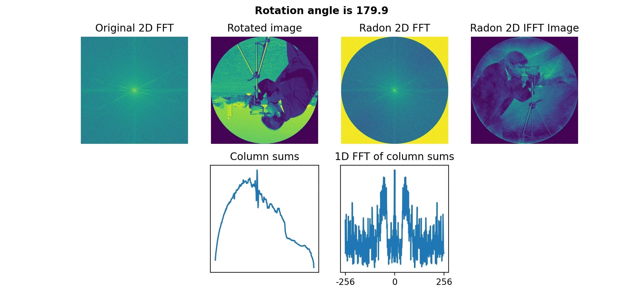
Now, let’s apply a 5° rotation and repeat the same process!

By collecting our line integrals offset by a rotation angle, we have now recovered a new orthogonal slice through our 2D FFT. A 2D IFFT recovers a slightly improved (but still terrible) approximation of the original image.
In the limit, though, if we repeat this process for lots of angles… we get the Radon transform! The Radon transform is the transform of our n-dimensional volume to a complete set of (n-1)-dimensional line integrals. The inverse Radon transform is the transform from our complete (n-1)-dimensional line integrals back to the original image. Under the hood, all of this is accomplished with the (inverse) Fourier transform!
As expected, repeating with closely spaced rotation angles recovers an accurate approximation of our original 2D FFT and a correspondingly accurate approximation of our original 2D image (Figure 3)!
Practical limitations
In reality, we don’t get the complete set. Instead, we are usually constrained by time, cost, or the negative impacts of additional images, e.g., giving a patient 10,000 x-ray scans is frowned upon 
Let’s take a look at the approximation we get from 5° rotational spacings (Figure 4)!
Remarkably, even though we have sparsely recovered values from 2D Fourier space, we have still recovered the key features of our image contents.
Conclusion
We now understand the basics principle of the Radon transform with respect to imaging! The (inverse) Radon transform describes a fundamental relationship between the Fourier transform of line integrals and the Fourier transform of the full-dimensional volume being imaged.
Up next, we will walk through the supporting code and explore the processing artifacts common to tomography. Thanks for reading; I hope you learned something!


