
Time is probably the most important dimension for metrics.
In the business world, business executives, analysts, and product managers track metrics over time.
In the startup world, VCs want metrics to grow 5% week-on-week.
In public stock markets, long-term investors evaluate metrics on a quarter-on-quarter basis to make buy/sell decisions. Short-term traders monitor stock prices at a much smaller time granularity – minutes or hours – to make the same decisions.
In the system monitoring world, teams track metrics on a second or a minute basis.
In the data science world, time series analysis is an important component of work.
Even though time may be the most important dimension in the data, data does have many other dimensions. These dimensions have varying cardinality. Some high cardinality dimensions can have thousands of unique dimension values.
It’s almost impossible to manually monitor metrics across thousands of these dimension values and their combinations. This is where timeseries analysis, particularly timeseries Anomaly Detection comes in handy.
Challenges in running anomaly detection on business data
- Most business Data is in SQL databases
Timeseries analysis needs timeseries data as an input. But most business data is tabular and sits in relational data warehouses and databases. Analysts typically use Sql to query these databases. How can we use SQL to generate timeseries data?
2. How to split metrics by dimensions?
Some dimensions can have thousands of unique dimension values. Running anomaly detection for all dimensions values will be expensive and noisy. How can we select significant dimension values only for our analysis?
3. Anomaly Detection at Scale is Expensive
Say you work for an online retailer. Your store sells 1000 products. You want to run anomaly detection on daily orders for each of these 1000 products. This means the following:
Number of Metrics = 1 (Orders) Number of Dimension Values = 1000 (1000 products) Number of Metric Combinations = 1000 (1 metric * 1000 dimension values)
This means the anomaly detection process must run 1000 times every day, once for each metric combination.
Let’s say you want to monitor Orders by another dimension – State (50 unique values). You also want to monitor the metric by the combinations of these two dimensions. This means the anomaly detection process must now run 51,050 times every day.
51,050 = (1 metric 1000 products) + (1 metric 50 states) + (1 metric 1000 products 50 states)
To get a sense of infrastructure pricing, let’s look at the pricing of the AWS anomaly detection service. AWS will charge you $638 per month to track 51K metric combinations on a daily basis.
This is what you will pay for just running the anomaly detection process. Before each run of the process, you need to run a query to pull data from your datawarehouse. 51K metric combinations mean 51K queries on your datawarehouse daily, which is an additional cost.
And this is just the cloud infrastructure cost.
4. Anomaly Detection at Scale is Noisy
Each of these 51K metric combinations has the potential to be an anomaly. Even if 0.1% of these combinations turn out to be anomalies, you are looking at 51 anomalies on a daily basis, for a single metric.
Will you or your team have the bandwidth to take action on so many anomalies every single day? Probably no.
If you don’t act on these anomalies, these anomalies don’t add any business value. Instead, they just add to your cost.
5. When an anomaly is detected, how to dig deeper and do root cause analysis?
Say you have the following anomaly:
Orders for State = CA decreased by 15% yesterday
This might raise questions like:
- Did the Orders decrease for all cities in the state? If not, which cities?
- Did the Orders decrease for all products or a specific few?
How can we answer these questions quickly?
Faced with these challenges, we started building CueObserve. Below is how we are solving these.
1. Create a Virtual Dataset
Datasets are similar to aggregated SQL VIEWS of data. We write a SQL GROUP BY query with aggregate functions to roll-up data, map its columns as dimensions and metrics, and save it as a virtual Dataset.
Below is a sample GROUP BY query for BigQuery:
2. Define an anomaly
We can now define one or more anomaly detection jobs on the dataset. The anomaly detection job can monitor a metric at an aggregate level or split the metric by a dimension.
When we split a metric by a dimension, we limit the number of unique dimension values. We use one of 3 ways to limit:
- Top N: limit based on the dimension value’s contribution to the metric.
- Min % Contribution: limit based on the dimension value’s contribution to the metric.
- Minimum Average Value: limit based on the metric’s average value.
3. Execute Dataset SQL
As the first step in the anomaly detection process, we execute the dataset’s SQL query and fetch the result as a Pandas dataframe. This dataframe acts as the source data for identifying dimension values and the anomaly detection process.
4. Generate Sub dataframes
Next, we create new dataframes on which the actual anomaly detection process will run. During this process, we find dimension values and create sub-dataframes by filtering on the dimension. The dimension values for which sub dataframes need to be created are determined by one of the 3 dimension split rules mentioned above. For example, if the dimension split rule is Top N, an internal method determines the Top N dimension values and returns a list of dicts, each containing the dimension value string, its percentage contribution, and the sub dataframe.
The sub dataframes mentioned are just dataframes after filtering for specific dimension values and removing all other columns except the timestamp column and metric column.
datasetDf[datasetDf[dimensionCol] == dimVal][[timestampCol, metricCol]]5. Aggregate Sub dataframes
One important step in the preparation of sub dataframes is the aggregation on timestamp which you can see in the previous code snippet.
"df": aggregateDf(tempDf, timestampCol)This aggregation involves grouping the filtered sub dataframe over the timestamp column and summing it over the metric column. We also rename the timestamp column as "ds" and the metric column as "y", as Prophet requires the dataframe columns to be named as such.
6. Generate Timeseries Forecast
We now feed the timeseries dataframe into Prophet. Each dataframe is separately trained on Prophet and a forecast is generated. Each dataframe must have at least 20 data points after aggregation as anything less than that would be too little training data for reasonably good results. There are some other considerations that are taken with respect to the granularity of the dataframe, like the number of predictions Prophet makes and also the training data interval. For hourly granularity, we only train Prophet on the last 7 days of data.
We initialize Prophet with predetermined parameters and interval width for reasonably broad confidence intervals. Later, we plan on making these settings configurable as well. After getting the confidence intervals and predicted values for the future, we clip all predicted values to be greater than zero and remove all extra columns from Prophet’s output.
7. Detect Anomaly
Next, we combine the actual data with the forecasted data from Prophet, along with the uncertainty interval bands. These bands estimate the trend of the data and will be used as the threshold for determining a data point as an anomaly. For each data point in the original dataframe, we check if it lies within the predicted bands or not and classify it as an anomaly accordingly.
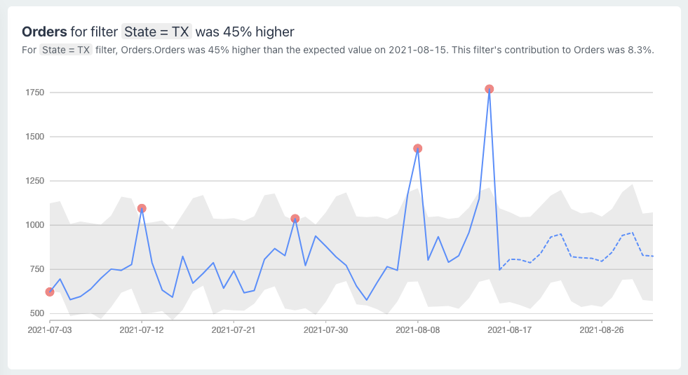
Finally, we store all the individual results of the process along with the metadata in a format for easy visual representation. Below is a sample anomaly visualization.
Conclusion
To run anomaly detection on multi-dimensional business data, we write a SQL GROUP BY query, map its columns as dimensions and measures, and save it as a virtual dataset. We then define one or more anomaly detection jobs on the dataset. We limit the number of dimension values to minimize noise and reduce infrastructure costs.
When an anomaly detection job runs, we execute the dataset SQL and store the result as a Pandas dataframe. We generate one or more timeseries from the dataframe. We then generate a forecast for each timeseries using Prophet. Finally, we create a visual card for each timeseries.


