Making Sense of Big Data
Markov Decision Process (MDP) is a foundational element of reinforcement learning (RL). MDP allows formalization of sequential decision making where actions from a state not just influences the immediate reward but also the subsequent state. It is a very useful framework to model problems that maximizes longer term return by taking sequence of actions. Chapter 3 of the book "Reinforcement Learning – An Introduction" by Sutton and Barto [1] provides an excellent introduction to MDP. The book is also freely available for download.
Expressing a problem as an MDP is the first step towards solving it through techniques like dynamic programming or other techniques of RL. A robot playing a computer game or performing a task are often naturally maps to an MDP. But many other real world problems can be solved through this framework too. Not many real world examples are readily available though. This article provides some real world examples of finite MDP. We also show the corresponding transition graphs which effectively summarizes the MDP dynamics. Such examples can serve as good motivation to study and develop skills to formulate problems as MDP.
MDP Basics
In an MDP, an agent interacts with an environment by taking actions and seek to maximize the rewards the agent gets from the environment. At any given time stamp t, the process is as follows
- The environment is in state St
- The agent takes an action At
- The environment generates a reward Rt based on St and At
- The environment moves to the next state St+1
The goal of the agent is to maximize the total rewards (ΣRt) collected over a period of time. The agent needs to find optimal action on a given state that will maximize this total rewards. The probability distribution of taking actions At from a state St is called policy π(At | St). The goal of solving an MDP is to find an optimal policy.
To express a problem using MDP, one needs to define the followings
- states of the environment
- actions the agent can take on each state
- rewards obtained after taking an action on a given state
- state transition probabilities.
The actions can only be dependent on the current state and not on any previous state or previous actions (Markov property). Rewards are generated depending only on the (current state, action) pair. Both actions and rewards can be probabilistic.
Once the problem is expressed as an MDP, one can use dynamic programming or many other techniques to find the optimum policy.
There are much more details in MDP, it will be useful to review the chapter 3 of Sutton’s RL book.
Real World Examples of MDP
1. Whether to fish salmons this year
We need to decide what proportion of salmons to catch in a year in a specific area maximizing the longer term return. Each salmon generates a fixed amount of dollar. But if a large proportion of salmons are caught then the yield of the next year will be lower. We need to find the optimum portion of salmons to catch to maximize the return over a long time period.
Here we consider a simplified version of the above problem; whether to fish a certain portion of salmon or not. This problem can be expressed as an MDP as follows
States: The number of salmons available in that area in that year. For simplicity assume there are only four states; empty, low, medium, high. The four states are defined as follows
Empty -> no salmons are available; low -> available number of salmons are below a certain threshold t1; medium -> available number of salmons are between t1and t2; high -> available number of salmons are more than t2
Actions: For simplicity assumes there are only two actions; fish and not_to_fish. Fish means catching certain proportions of salmon. For the state empty the only possible action is not_to_fish.
Rewards: Fishing at certain state generates rewards, let’s assume the rewards of fishing at state low, medium and high are $5K, $50K and $100k respectively. If an action takes to empty state then the reward is very low -$200K as it require re-breeding new salmons which takes time and money.
State Transitions: Fishing in a state has higher a probability to move to a state with lower number of salmons. Similarly, not_to_fish action has higher probability to move to a state with higher number of salmons (excepts for the state high).
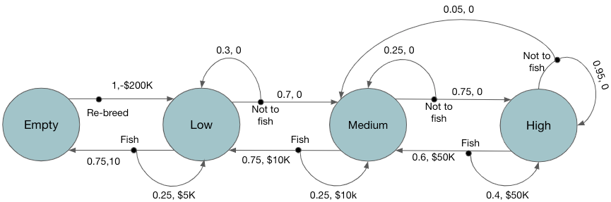
Figure 1 shows the transition graph of this MDP. There are two kinds of nodes. Large circles are state nodes, small solid black circles are action nodes. Once an action is taken the environment responds with a reward and transitions to the next state. Such state transitions are represented by arrows from the action node to the state nodes. Each arrow shows the <transition probability, reward>. For example, from the state Medium action node Fish has 2 arrows transitioning to 2 different states; i) Low with (probability=0.75, reward=$10K) or ii) back to Medium with (probability=0.25, reward=$10K). In the state Empty, the only action is Re-breed which transitions to the state Low with (probability=1, reward=-$200K).
2. Quiz Game Show
In a quiz game show there are 10 levels, at each level one question is asked and if answered correctly a certain monetary reward based on the current level is given. Higher the level, tougher the question but higher the reward.
At each round of play, if the participant answers the quiz correctly then s/he wins the reward and also gets to decide whether to play at the next level or quit. If quit then the participant gets to keep all the rewards earned so far. At any round if participants failed to answer correctly then s/he looses "all" the rewards earned so far. The game stops at level 10. The goal is to decide on the actions to play or quit maximizing total rewards
States: {level1, level2, …, level10}
Actions: Play at next level or quit
Rewards: Play at level1, level2, …, level10 generates rewards $10, $50, $100, $500, $1000, $5000, $10000, $50000, $100000, $500000 with probability p = 0.99, 0.9, 0.8, …, 0.2, 0.1 respectively. The probability here is a the probability of giving correct answer in that level. At any level, the participant losses with probability (1- p) and losses all the rewards earned so far.
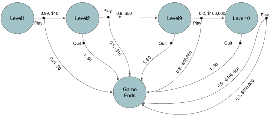
In Figure 2 we can see that for the action play, there are two possible transitions, i) won which transitions to next level with probability p and the reward amount of the current level ii) lost which ends the game with probability (1-p) and losses all the rewards earned so far. Action quit ends the game with probability 1 and no rewards.
3. Reducing wait time at a traffic intersection
We want to decide the duration of traffic lights in an intersection maximizing the number cars passing the intersection without stopping. For simplicity, lets assume it is only a 2-way intersection, i.e. traffic can flow only in 2 directions; north or east; and the traffic light has only two colors red and green. Also assume the system has access to the number of cars approaching the intersection through sensors or just some estimates.
Say each time step of the MDP represents few (d=3 or 5) seconds. At each time step we need to decide whether to change the traffic light or not.
States: A state here is represented as a combination of
- The color of the traffic light (red, green) in each directions
- Duration of the traffic light in the same color
- The number of cars approaching the intersection in each direction.
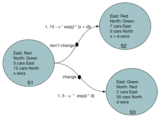
Actions: Whether or not to change the traffic light
Rewards: Number of cars passing the intersection in the next time step minus some sort of discount for the traffic blocked in the other direction. The discount should exponentially grow with the duration of traffic being blocked. Note that the duration is captured as part of the current state and therefore the Markov property is still preserved.
Reward = (number of cars expected to pass in the next time step) – α exp( β duration of the traffic light red in the other direction)
State Transitions: Transitions are deterministic. Action either changes the traffic light color or not. For either of the actions it changes to a new state as shown in the transition diagram below.
4. How many patients to admit
A hospital has a certain number of beds. It receives a random number of patients everyday and needs to decide how many patients it can admit. Also, everyday certain portion of patients in the hospital recovers and released. The hospital would like to maximize the number of people recovered over a long period of time.
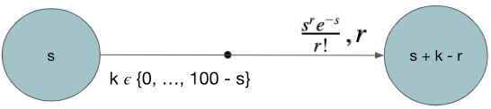
States: The number of available beds {1, 2, …, 100} assuming the hospital has 100 beds
Action: Each day the hospital gets requests of number of patients to admit based on a Poisson random variable. The action is the number of patients to admit. Therefore the action is a number between 0 to (100 – s) where s is the current state i.e. the number of beds occupied. The action needs to be less than the number of requests the hospital has received that day.
So action = {0, min(100 – s, number of requests)}
Rewards: The reward is the number of patient recovered on that day which is a function of number of patients in the current state. We can treat this as a Poisson distribution with mean s.
Conclusions
In this doc, we showed some examples of real world problems that can be modeled as Markov Decision Problem. Such real world problems show the usefulness and power of this framework. These examples and corresponding transition graphs can help developing the skills to express problem using MDP. As further exploration one can try to solve these problems using dynamic programming and explore the optimal solutions.
References
[1] Reinforcement Learning: An Introduction by Richard S. Sutton and Andrew G. Barto


