In this post, I want to show an interesting result that was not obvious to me at first, which is the following:
Linear regression and linear-kernel ridge regression with no regularization are equivalent.
There are actually a lot of concepts and techniques involved here, so we will review each one by one, and finally use them all to explain this statement.
First, we’ll review the classic linear regression. Then I’ll explain what the Kernel trick is and the linear-kernel, and finally we’ll show a mathematical proof for the statement above.
A quick reminder of the classic Linear Regression
The maths of linear regression
The classic – Ordinary Least Squares or OLS- linear regression is the following problem:

where:
- Y is a vector of length n and consists of the target value of the linear model
- beta is a vector of length m: this is the unknown the model will have to "learn"
- X is the data matrix with shape n rows and m columns. We often say that we have n vectors recorded in the m-features space
So the goal is to find the values of beta that minimizes the squared errors:

This problem actually has a closed form solution, and is known as the Ordinary Least Squares problem. The solution is:

Once the solution is known, we can use the fitted model to compute new Y-values given new X-values using:

Python for linear regression
Let’s verify our math with scikit-learn: here is a python code that gives an example of a linear regression, using sklearn linear regressor, as well as a numpy-based regression
%matplotlib qt
import numpy as np
import matplotlib.pyplot as plt
from sklearn.linear_model import LinearRegression

np.random.seed(0)
n = 100
X_ = np.random.uniform(3, 10, n).reshape(-1, 1)
beta_0 = 2
beta_1 = 2
true_y = beta_1 * X_ + beta_0
noise = np.random.randn(n, 1) * 0.5 # change the scale to reduce/increase noise
y = true_y + noise

fig, axes = plt.subplots(1, 2, squeeze=False, sharex=True, sharey=True, figsize=(18, 8))
axes[0, 0].plot(X_, y, "o", label="Input data")
axes[0, 0].plot(X_, true_y, '--', label='True linear relation')
axes[0, 0].set_xlim(0, 11)
axes[0, 0].set_ylim(0, 30)
axes[0, 0].legend()

# f_0 is a column of 1s
# f_1 is the column of x1
X = np.c_[np.ones((n, 1)), X_]

beta_OLS_scratch = np.linalg.inv(X.T @ X) @ X.T @ y
lr = LinearRegression(
    fit_intercept=False, # do not fit intercept independantly, since we added the 1 column for this purpose
).fit(X, y)

new_X = np.linspace(0, 15, 50).reshape(-1, 1)
new_X = np.c_[np.ones((50, 1)), new_X]
new_y_OLS_scratch = new_X @ beta_OLS_scratch
new_y_lr = lr.predict(new_X)
axes[0, 1].plot(X_, y, 'o', label='Input data')
axes[0, 1].plot(new_X[:, 1], new_y_OLS_scratch, '-o', alpha=0.5,  label=r"OLS scratch solution")
axes[0, 1].plot(new_X[:, 1], new_y_lr, '-*', alpha=0.5, label=r"sklearn.lr OLS solution")
axes[0, 1].legend()
fig.tight_layout()
print(beta_OLS_scratch)
print(lr.coef_)
[[2.12458946]
[1.99549536]]
[[2.12458946 1.99549536]]As you can see, both methods give identical results (duh!):

Kernel-trick
Lets now review a common technique known as the Kernel Trick.
The idea is the following:
Our original problem (can be anything like classification or regression) lives in the space of the input data matrix X, of shape n-vectors in a m-features space. Sometimes, the vectors cannot be separated or classified in this low dimension space, so we want to transform the input data to a high dimension space. We can do this by hand, by creating new features manually. As the number of feature grows, the numerical computation will increase as well: imagine computing the dot product of 2 vectors of length 1 billion, and repeat for all vectors in your matrix.
The kernel trick consists in using well-designed transformation functions – usually noted T or phi – that creates a new vector x’ of length m’ from a vector x of length m, such that our new data will indeed have high dimension, but by keeping the computation load to a minimum.
To achieve this, the function phi must fill some properties, such that the dot product in the new high dimension feature-space can be written as a function – the kernel function- of the corresponding input vectors:

What this means is that the inner product in the high dimension space can be expressed as a function of the input vectors. In other words, we can compute the inner product in the high dimension space only using the low dimension vectors. That is the kernel trick: we can benefit from the high-dimension space versatility, while never actually doing any computation there.
The only condition is that we only need the dot product in the high-dimension space.
There are actually powerful mathematical theorems that describe what are the conditions to create such transformation phi and/or such kernel functions.
Examples of kernel functions
A first example of kernel to create a m^2 dimension space from a m dimension is by using the following:

Another example: adding a constant in the kernel function increases the number of dimension, with new features that are scaled input features:

Another kernel that we’ll use below is the linear-kernel:

So the identity transformation is equivalent to using a kernel function that compute the inner product in the original space.
There are actually a lot of other useful kernels, like the radial (RBF) kernel or the more general polynomial kernel, that create high-dimension AND non-linear feature spaces. For completeness, here is an example of using RBF kernel to compute non-Linear Regression in a linear regression context:
import numpy as np
from sklearn.kernel_ridge import KernelRidge
import matplotlib.pyplot as plt

np.random.seed(0)
X = np.sort(5 * np.random.rand(80, 1), axis=0)
y = np.sin(X).ravel()
y[::5] += 3 * (0.5 - np.random.rand(16))

# Create a test dataset
X_test = np.arange(0, 5, 0.01)[:, np.newaxis]

# Fit the KernelRidge model with an RBF kernel
kr = KernelRidge(
    kernel='rbf', # use RBF kernel
    alpha=1, # regularization
    gamma=1, # scale for rbf
)
kr.fit(X, y)

y_rbf = kr.predict(X_test)

# Plot the results
fig, ax = plt.subplots()
ax.scatter(X, y, color='darkorange', label='Data')
ax.plot(X_test, y_rbf, color='navy', lw=2, label='RBF Kernel Ridge Regression')
ax.set_title('Kernel Ridge Regression with RBF Kernel')
ax.legend()

The linear-kernel in linear regression
If the transformation phi transforms x to phi(x), then we can write a new linear regression problem:

Notice how the dimensions change: the input matrix for the linear regression problem goes from [nxm] to [nxm’], so the coefficient vector beta goes from length m to m’.
And this where the kernel trick appears: when computing the solution beta’, notice that the product of X’ with its transpose appears, which is actually the matrix of all the dot product, called the Kernel matrix for obvious reasons:

Linear-kernelized and linear regression
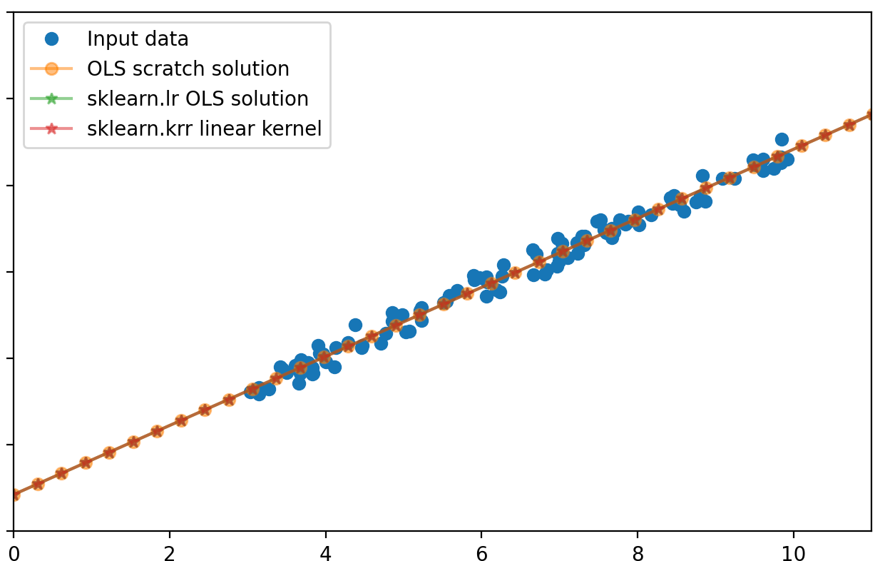
Finally, lets see a proof of the original statement: that using the linear-kernel in a linear regression is useless as it is equivalent to standard linear regression.
Linear-kernel is usually used in the context of Support Vector Machines, but I was wondering how it would perform in linear regression.
To show that both approaches are equivalent, we have to proove that:

The first method using beta is the original linear regression, and the second using beta’ is using linear-kernalized approach.
We can prove this actually using matrix properties and relations seen above:

We can verify this again using python and scikit learn:
%matplotlib qt
import numpy as np
import matplotlib.pyplot as plt
from sklearn.linear_model import LinearRegression

np.random.seed(0)
n = 100
X_ = np.random.uniform(3, 10, n).reshape(-1, 1)
beta_0 = 2
beta_1 = 2
true_y = beta_1 * X_ + beta_0
noise = np.random.randn(n, 1) * 0.5 # change the scale to reduce/increase noise
y = true_y + noise

fig, axes = plt.subplots(1, 2, squeeze=False, sharex=True, sharey=True, figsize=(18, 8))
axes[0, 0].plot(X_, y, "o", label="Input data")
axes[0, 0].plot(X_, true_y, '--', label='True linear relation')
axes[0, 0].set_xlim(0, 11)
axes[0, 0].set_ylim(0, 30)
axes[0, 0].legend()

# f_0 is a column of 1s
# f_1 is the column of x1
X = np.c_[np.ones((n, 1)), X_]

beta_OLS_scratch = np.linalg.inv(X.T @ X) @ X.T @ y
lr = LinearRegression(
    fit_intercept=False, # do not fit intercept independantly, since we added the 1 column for this purpose
).fit(X, y)

new_X = np.linspace(0, 15, 50).reshape(-1, 1)
new_X = np.c_[np.ones((50, 1)), new_X]
new_y_OLS_scratch = new_X @ beta_OLS_scratch
new_y_lr = lr.predict(new_X)
axes[0, 1].plot(X_, y, 'o', label='Input data')
axes[0, 1].plot(new_X[:, 1], new_y_OLS_scratch, '-o', alpha=0.5,  label=r"OLS scratch solution")
axes[0, 1].plot(new_X[:, 1], new_y_lr, '-*', alpha=0.5, label=r"sklearn.lr OLS solution")
axes[0, 1].legend()
fig.tight_layout()
print(beta_OLS_scratch)
print(lr.coef_)
Wrapup
In this post we reviewed the simple linear regression, including the matrix formulation of the problem and its solution.
We then saw what the kernel trick is and how it allows us to benefit from very high dimension space without actually moving our low dimension data to this computation-intensive space.
Finally, I showed that the linear-kernel in the context of linear regression is actually useless and correspond to the simple linear regression.
If you’re considering joining Medium, use this link to quickly subscribe and become one of my referred member :
and subscribe to get an notification when I publish new post:
Finaly, you can check out some of my other post, on Fourier transform, pandas dtypes, or linear algebra techniques for datascience:
Fourier-transform for time-series : detrending
PCA/LDA/ICA : a components analysis algorithms comparison
PCA-whitening vs ZCA-whitening : a numpy 2d visual
300-times faster resolution of Finite-Difference Method using numpy


