Introduction to Image Processing with Python — Image Filtering
Edge Detection and Other Morphological Operators for Beginners

In this article, we will tackle basic image filtering. We will see how to apply kernels to an image to change its overall look. Though this can be utilized for purely aesthetic purposes, we will also go through the practical applications of image filtering.
Let’s get started!
As always we begin by importing the required Python Libraries
import numpy as np
import matplotlib.pyplot as plt
from skimage.io import imread, imshow
from skimage.color import rgb2gray
from skimage import img_as_uint
from scipy.signal import convolve2d
Great, now the next step is to define our filters (going forward referred to as Kernels as is the nomenclature). To start off let us first define a simple edge detection kernel.
kernel_edgedetection = np.array([[-1, -1, -1],
                                 [-1, 8.5, -1],
                                 [-1, -1, -1]])
As you may recall in my previous article, images are represented as matrices. In this case, our kernel is defined as a 3x3 matrix.
imshow(kernel_edgedetection, cmap = 'gray');
Now let us apply this to our image. Below is the image we shall be using as an example.
morph = imread('Morph_Image_1.png')
To apply the edge detection kernel to our image we simply have to use the convolve2d function in SciPy. But before that, we must first convert our image into greyscale (remember that we are applying a 2 Dimensional kernel).
plt.figure(num=None, figsize=(8, 6), dpi=80)
morph_gray = rgb2gray(morph)
imshow(morph_gray);
To apply the kernel, we can simply use the convolve2d function in SciPy.
conv_im1 = convolve2d(morph_gray, kernel_edgedetection)
imshow(abs(conv_im1) , cmap='gray');
As we can see, the application of the kernel highlights all the edges detected by the machine. Note that there is no hard rule on the exact figures to use for edge detection. The main idea is that you have to define a kernel that will search for contrasts in the image. To explore this idea, let us create a function that uses different figures for edge detection.
def edge_detector(image):
    f_size = 15
    morph_gray = rgb2gray(image)
    kernels = [np.array([[-1, -1, -1],
                         [-1, i, -1],
                        [-1, -1, -1]]) for i in range(2,10,1)]

    titles = [f'Edge Detection Center {kernels[k][1][1]}' for k in
              range(len(kernels))]

    fig, ax = plt.subplots(2, 4, figsize=(17,12))

    for n, ax in enumerate(ax.flatten()):
        ax.set_title(f'{titles[n]}', fontsize = f_size)
        ax.imshow(abs(convolve2d(morph_gray, kernels[n])) ,
                  cmap='gray')
        ax.set_axis_off()

    fig.tight_layout()
Apologies for the rather dense code as it may be difficult to understand for beginners, but I found it pertinent to create due to the number of subplots. In further lessons, I will give tips on how to create flat codes as well.
Going back to the image, we can see that the sweet spot for the edge value seems to be between 7 and 9. One could theoretically go deeper into the most visually appealing value but let us just say that 8 is the best value to use.
Note that so far we have only used the edge detection kernel, let us also take a look at two other popular kernels known as the Vertical Sobel and Horizontal Sobel.
# Horizontal Sobel Filter
h_sobel = np.array([[1, 2, 1],
                    [0, 0, 0],
                    [-1, -2, -1]])# Vertical Sobel Filter
v_sobel = np.array([[1, 0, -1],
                    [2, 0, -2],
                    [1, 0, -1]])fig, ax = plt.subplots(1, 2, figsize=(17,12))ax[0].set_title(f'Horizontal Sobel', fontsize = 15)
ax[0].imshow(h_sobel, cmap='gray')
ax[0].set_axis_off()ax[1].set_title(f'Vertical Sobel', fontsize = 15)
ax[1].imshow(v_sobel , cmap='gray')
ax[1].set_axis_off()

The kernels look specifically for horizontal and vertical edges specifically.
fig, ax = plt.subplots(1, 2, figsize=(17,12))ax[0].set_title(f'Horizontal Sobel', fontsize = 15)
ax[0].imshow(abs(convolve2d(morph_gray, h_sobel)), cmap='gray')
ax[0].set_axis_off()ax[1].set_title(f'Vertical Sobel', fontsize = 15)
ax[1].imshow(abs(convolve2d(morph_gray, v_sobel)) , cmap='gray')
ax[1].set_axis_off()

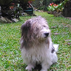
As we can see, there are many fascinating filters we can work with. I just chose edge detection as it the most understandable for beginners and other people who are just getting into image processing. To close this article out, let us apply these filters to a much more complex image.

Applying an edge filter to the image does not yield very good results.
kernel_edgedetection = np.array([[-1, -1, -1],
                                 [-1, 8.5, -1],
                                 [-1, -1, -1]])
edge_dog = abs(convolve2d(graydog, kernel_edgedetection,
               mode = 'valid'))
imshow(edge_dog, cmap='gray');
Though we can see that the dog is detectable, we also see that the machine picks up “edges” in the sand. Indeed it is rendering them as a grid pattern. To remedy this we can first blur the image.
blur = (1 / 16.0) * np.array([[1., 2., 1.],
                                 [2., 4., 2.],
                                 [1., 2., 1.]])
blurred_dog = abs(convolve2d(graydog, blur, mode = 'valid' ))
imshow(blurred_dog , cmap='gray');
From here we can convolve the image with the edge detector. Yielding the below result.
kernel_edgedetection = np.array([[-1, -1, -1],
                                 [-1, 8.05, -1],
                                 [-1, -1, -1]])blurry_edge_dog = abs(convolve2d(blurred_dog, kernel_edgedetection,
                      mode = 'valid'))
imshow( blurry_edge_dog , cmap='gray');

We see that the sand no longer exhibits edges as before, a good improvement that will help the machine not fall prey to false (or irrelevant) patterns.
Lastly, we would like to see the shape of the dog. Notice how the dog is actually much darker than the surrounding sand, we can use this to our advantage. We simply need to transform the matrix into integers and then filter out all the pixels that are less than the mean.
binary_dog = img_as_uint(blurry_edge_dog < np.mean(blurry_edge_dog))
imshow(binary_dog , cmap='gray');
Though still grainy, the shape of the dog becomes easy to spot. The grains of sand also retain their noise like quality.
In Conclusion
Though we used kernels to do some pretty mundane things (detecting vertical and horizontal edges, finding the shapes of dogs), knowing how to use them correctly can be vital in your journey as a data scientist. As we have learned, some images may be easier to filter than others (particularly images with very well defined patterns).
Remember that despite their parallels, our human minds interpret images very differently from our machines. Patterns that we usually ignore (such as lines in the sand) may be treated as important by the machine. In our case we had to first blur the image before enacting the proper filters, this is not too different from the way our own brains “junk” visual information. Just be aware that programming filters in the machine will help it see the world the way we want it to see.
Equally as important though, be aware that we as humans also see the world based on our own filters. And that we too were programmed to see the world the way someone else wanted to us to see it.