Introduction to Image Processing with Python — Image Representation for Beginners

Processed Doggo (Image by Author)

Image Processing using Python is a fun way to understand how pictures can be represented via math and code. I hope that this short article can give you an idea of how your machines understand image data.

Let’s get started.

# First import the required Python Libraries
import numpy as np
import matplotlib.pyplot as plt
from skimage import img_as_uint
from skimage.io import imshow, imread
from skimage.color import rgb2hsv
from skimage.color import rgb2gray

Great! Now that we have imported the required libraries, we can begin with the basics. An image can be thought of as a matrix where every pixel’s color is represented by a number on a scale.

array_1 = np.array([[255, 0], 
                    [0, 255]])
imshow(array_1, cmap = 'gray');

Output 1

The above output is a visual representation of the matrix we just created. Note that we are not limited to a simple 2x2 matrix. Below is an example of a 3x3 matrix.

array_2 = np.array([[255, 0, 255], 
                    [0, 255, 0],
                    [255, 0, 255]])
imshow(array_2, cmap = 'gray');

Output 2

Although our examples were picking colors on the extreme end of the spectrum, we can also access any of the colors in between.

Remember that you do not have to manually encode each number!

The below image was constructed with the use of the arange function of NumPy and created another image by getting the transpose of the first one.

array_spectrum = np.array([np.arange(0,255,17), 
                   np.arange(255,0,-17),
                   np.arange(0,255,17),
                   np.arange(255,0,-17)])
fig, ax = plt.subplots(1, 2, figsize=(12,4))
ax[0].imshow(array_spectrum, cmap = 'gray')
ax[0].set_title('Arange Generation')
ax[1].imshow(array_spectrum.T, cmap = 'gray')
ax[1].set_title('Transpose Generation');

Output 3

For simplicity we have been using grayscale, but please remember that the machine actually understands colors as different mixtures of Red, Green, and Blue. As such, we can represent images as 3 dimensional matrixes. Each pixel being represented as a Python list that specifies their color mix.

array_colors = np.array([[[255, 0, 0], 
                         [0, 255, 0],
                         [0, 0, 255]]])
imshow(array_colors);

Output 4

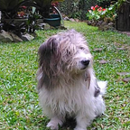
Let’s try manipulating an actual image. Below is an image of a loveable doggo.

doggo = imread('doggo.png')
imshow(doggo);

Doggo Image (Image by Author)

doggo.shape

Size of Doggo Image

Checking for the size of the image, we see that it is a 390 x 385 x 3 matrix. Remember that using Python we can slice this matrix and represent each section as its own image box.

fig, ax = plt.subplots(1, 3, 
                       figsize=(6,4), 
                       sharey= True)
    
ax[0].imshow(doggo[:, 0:130])
ax[0].set_title('First Split')
    
ax[1].imshow(doggo[:, 130:260])
ax[1].set_title('Second Split')
    
ax[2].imshow(doggo[:, 260:390])
ax[2].set_title('Third Split');

Split Doggo

Remember that although you can do this for all images, each image will have different dimensions. Essentially what I did was find the dimensions that would split my image into 3 equal parts. Depending on the dimensions of your image, you will have to specify different figures.

Below are the specifications for the dog’s face.

imshow(doggo[95:250, 130:275]);

Face Doggo

Now lets have some fun!

Remember that previously we stated that an image can be represented by a 3 dimensional matrix with each list specifying the color mix.

Matrix Doggo

Each row represents the specific pixel color, we can actually call each of the numbers individually. The numbers can then give us a representation of the image’s Red, Green, and Blue components.

fig, ax = plt.subplots(1, 3, figsize=(12,4), sharey = True)
ax[0].imshow(doggo[:,:,0], cmap='Reds')
ax[0].set_title('Red')
ax[1].imshow(doggo[:,:,1], cmap='Greens')
ax[1].set_title('Green')
ax[2].imshow(doggo[:,:,2], cmap='Blues')
ax[2].set_title('Blue');

RGB Doggo

Additionally, we can convert the image from RGB (Red, Green, Blue) to HSV (Hue, Saturation, Value).

This will give us the aforementioned figures for Hue, Saturation, and Value.

doggo_hsv = rgb2hsv(doggo)
fig, ax = plt.subplots(1, 3, figsize=(12,4), sharey = True)
ax[0].imshow(doggo_hsv[:,:,0], cmap='hsv')
ax[0].set_title('Hue')
ax[1].imshow(doggo_hsv[:,:,1], cmap='gray')
ax[1].set_title('Saturation')
ax[2].imshow(doggo_hsv[:,:,2], cmap='gray')
ax[2].set_title('Value');

HSV Doggo

Lastly, we can also convert the image matrix to grayscale. By we transform the image to a simple 2x2 matrix. This allows us to easily filter our image based on each pixel’s relation to a specified value.

doggo_gray = rgb2gray(doggo)
fig, ax = plt.subplots(1, 5, figsize=(17,6), sharey = True)
ax[0].imshow(doggo_gray, cmap = 'gray')
ax[0].set_title('Grayscale Original')
ax[1].imshow(img_as_uint(doggo_gray > 0.25), 
             cmap = 'gray')
ax[1].set_title('Greater than 0.25')
ax[2].imshow(img_as_uint(doggo_gray > 0.50), 
             cmap = 'gray')
ax[2].set_title('Greater than 0.50');
ax[3].imshow(img_as_uint(doggo_gray > 0.75), 
             cmap = 'gray')
ax[3].set_title('Greater than 0.75');
ax[4].imshow(img_as_uint(doggo_gray > np.mean(doggo_gray)), 
             cmap = 'gray')
ax[4].set_title('Greater than Mean');

Binary Doggo

That should give you a basic understanding of how to load and manipulate images using Python. To get a better understanding of image processing, it would be best if you could play around with the codes. I’d also encourage you to start by processing images of topics you actually like. In my case nature has always been a great source of inspiration.