
Linear regression is probably the most basic topic in statistical learning. Almost all courses in machine learning, statistics and econometrics start with the fundamentals of Ordinary Least Squares. And why not? Its defining equation _y = β_₀+β₁x + e seems easy enough. But why would you care about the OLS equation? Granted, in the days of large language models and self-driving cars, talking about linear regression sounds almost arcane. And yet, as we will see in this article, sometimes a flavour of linear regression is exactly what you need.
One of the advantages of linear regression is explainability. In our equation above, we can say that the impact of x on y is, on average, β₁, allowing for some random noise, e, and a constant term, _β₀._ However, this simple interpretation is underpinned by strong assumptions on how the data is generated: is the relation between x and y actually linear? Are we measuring x and y properly? Are we even seeing a representative sample of our target population? As you may have guessed, the answer to those questions tends to be No in real life. Which leads me to the use case that I want to present in this article: the Tobit model for censored data.
Gig economy meets censored data
Note: This article uses simulated data. This data is meant to be representative of a real-life scenario, but it does not contain any real transactions from any company mentioned in the article nor does it reflect their actual state of operations.Imagine that you are a data scientist at firm in the gig industry. Let’s say your company runs a riding app such as Uber. (This can apply to any match-making business, from food delivery, to home services or transportation.) Your manager wants to know what is the impact of offered rates on the number of rides a driver completes in a day. You’ve got a dataset that contains how many rides drivers completed after logging into the app in a day, including if those drivers who didn’t complete any. The dataset also contains a variable on earnings, which has been normalised by hour so that rides are comparable. "Easy – you think to yourself – I’ll just run a linear regression and thake the beta". Are you sure? Look at the chart below. It shows how many rides drivers in a city completed as a function of hourly earnings. Anything strange?
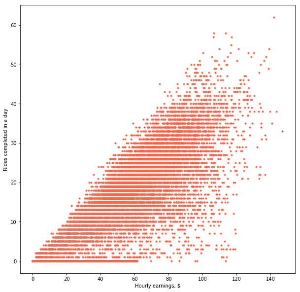
At first sight, not really. While there is a lot of variation, there seems to be a positive correlation between hourly earnings and number of rides completed. In other words, drivers work more if they are paid more. Economics 101. But let’s unpack the data a bit more. Look at the histogram below. It shows the distribution of rides completed per day per driver. As you can see, there’s a big agglomeration of points for 0 rides.
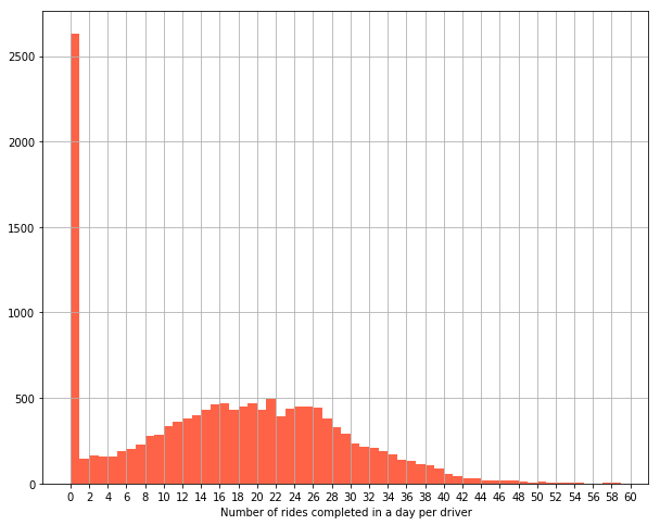
Now look at the scatter plot again. Doesn’t it feel like the cloud wants to continue on the negative side of the x-axis? "But this wouldn’t make sense – you think – You can’t do negative rides in a day!" And that’s true, you can’t. But your data is not necessarily faulty either. On the contrary, this is a well-known phenomenon in the field of Economics. What we are seeing here is a case of data censoring: drivers only complete a ride if they are willing to do so at a particular rate. However, some other drivers will have logged into the app, looked at the rates being paid at that time and decided that they are not worth their time. These are the ones who did zero rides.
The Tobit model
"What do you mean, less than nothing?" replied Wilbur. "I don’t think there is any such thing as less than nothing. Nothing is absolutely the limit of nothingness. It’s the lowest you can go. It’s the end of the line. How can something be less than nothing? If there were something that was less than nothing, then nothing would not be nothing, it would be something even though it’s just a very little bit of something. But if nothing is nothing, then nothing has nothing that is less than it is."
- James Tobin’s 1958 quote of E.B. White’s Charlotte’s Web (1952)
This problem was first identified by James Robin who, in his 1958 paper [1], studied the case of individual expenditure on durable goods. In particular, he noticed that his sample of American households showed that most of them would report zero consumption of automobiles or durable goods, as they couldn’t afford them. In other words, his sample necessarily had a lower limit at zero. He cleverly represented this problem in figure 1 of his paper, shown below.
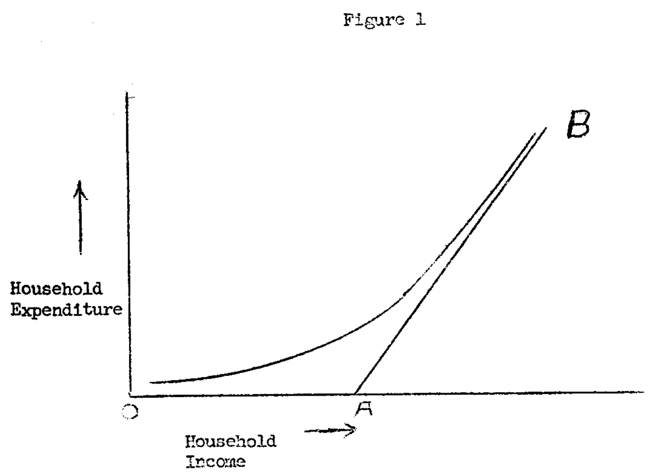
Notice the important implications for your OLS estimator. If you were to run a simple linear regression, your β₁ would be inconsistent, because your observed data is not distributed linearly across the chart. If we take Tobin’s image above, you would want an estimated β₁ for the slope of the line that goes from A to B – in other words, the unconditional average relationship between x and y. However, because your data is censored, the observed relation (the conditional average) is not linear, but something like the line between O and B. Basically, your model would be seeing far too many zeros for certain hourly rates, which should in reality be negative values if we allowed for "negative rides" to maintain the linear relationship (i.e. if we let the data cloud continue into the negative values of the y-axis). Therefore, because our sample is censored at zero rides, the data will not allow us to draw the true straight line that represents the linear relationship between x and y.
In his paper, Tobin proposed a method for the estimation of β₁ with censored data, which in time would come to be known as the Tobit model. His idea was to correct the way we estimate β₁ by accounting for the probability that an observation is censored at 0 (or at any other value, from below or from above). Why Tobit model and not Tobin model, you ask? The term was coined by Arthur Goldberger, another economist. It is the combination of the words Tobit and and probit, the classification technique used to calculate the probability that an observation is censored.
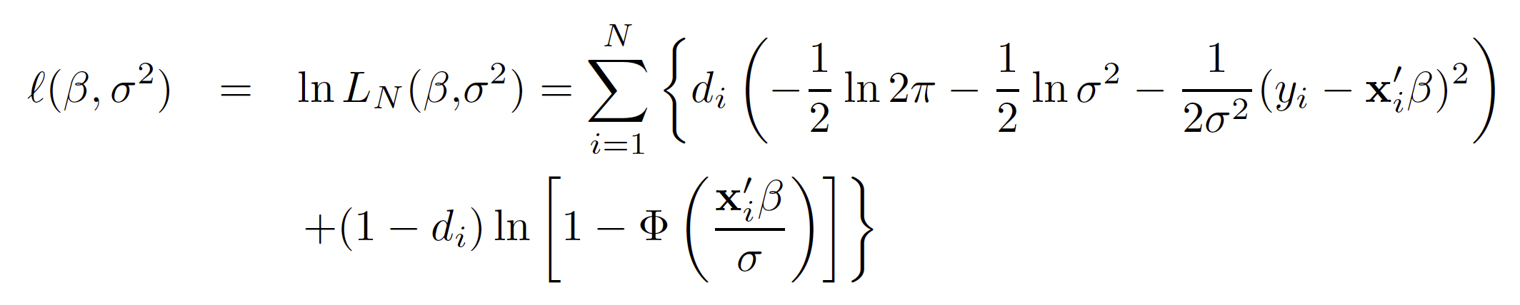
While the derivation of the model is beyond the scope of this article, let’s have a quick look at the problem for completeness. The function below shows the maximisation problem that we have to solve by maximum likelihood estimation to get to our true β₁ (shown in vector notation as β, together with _β₀)._ Tobin’s solution implies that errors are independent and normally distributed, with standard deviation σ. In the function, dᵢ would take value 0 if y = 0, and 1 otherwise. Thus, the left-hand side of the sum (the one multiplied by dᵢ, on the top line) is equivalent to the OLS likelihood function, whereas the right-hand side (multiplied by (1-dᵢ), bottom line), accounts for the probability that observation i is censored.
Implementation
Cool as it is, to the best of my knowledge there is no Python package to use the Tobit model in Python (at least I haven’t seen any on pip or conda). However, I found James Jensen’s implementation quite useful. I forked my own version of it, which you can find here, and I highly encourage you to do the same!
Remember that I said that β₁ would be inconsistent if we estimated it by simple OLS? In mathematical terms, that means that our estimate of β will not converge to its actual value. More simply, the slope of our linear relationship will be off. To illustrate what that would look like, the green line in the chart below shows the OLS fitted values in our drivers example. On the other hand, estimating β using the Tobit model gives us a slightly higher value (0.35 vs 0.33), which is represented by the blue line.
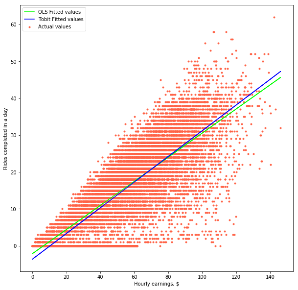
The difference between the OLS and the Tobit estimate can vary depending on your model specification – sometimes it’ll be bigger, sometimes it’ll be smaller. Notice that we haven’t included any control variables in our equation, nor do we have any solid identification strategy underpinning it. This means that our model could be improved, which would likely impact our estimates. Hence, we shouldn’t try to derive any meaning from these particular numbers.
Marginal effects
Now that you have run your Tobit model and come up with an estimate for β₁, you may be tempted to say that each driver will complete β₁ more rides for each additional dollar. But it’s not so simple! Let’s see why.
Generally speaking, our aim is to estimate the average impact of a change in earnings on rides completed. This is what economists call a "marginal effect". While we will skip mathematical details, this is equivalent to the derivate of y (rides) with respect to x (earnings) in our equation. In the OLS model, this is simply β₁. However, in the Tobit model, the marginal effect of x on y is slightly more complicated. Because we included the probability that an observation is censored in our derivation of β₁, we need to account for it in our interpretation of it as well.
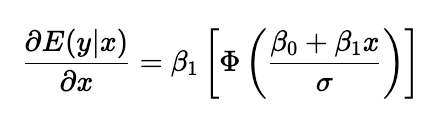
The equation above shows how a change in earnings translates into rides completed on average – hence the conditional expectation on the left hand side. On the right-hand side, we’ve got our β₁, multiplied by the cummulative distribution function (CDF, represented by Φ) of the Normal distribution evaluated at our model’s estimated value for y, that is, _β_₀+β₁x, and normalised by our error’s standard deviation, σ.
What I just described above may sound complicated, but you’ll see it actually isn’t. What the equation for the marginal effect means is that the average impact of a change in hourly earnings indeed depends on β₁. However, the coefficient is weighted by the probability that an individual is willing to work at the present hourly rate, as represented by the CDF. In other words, the marginal effect of offering an extra dollar will be different depending on whether that ride was originally $10 or $40. This makes sense if you think about it: the probability that someone works for $40 is probably higher than working for $10!
To see how this works in practice, let’s return to our Python implementation. To calculate marginal effects, I created a function, called margins, that builds on top of James Jensen’s solution. With our estimated β₁ of 0.35 and a starting hourly earnings rate of $10, the estimated marginal effect would be 0.17. Changing the starting rate to $40, however, yields a marginal effect of 0.32. If we take the hourly earnigs further up, say $100, the marginal effect is already 0.35. As you can see, the higher the earnings, the closer our marginal effect gets to β₁, as it is more likely for a driver to be willing to complete a ride for higher hourly earnings.
Conclusion
In this article we have seen how some apparently simple regression problems may actually get tricky if our observed data is censored. This is the case for companies in the Gig Economy industry, who may want to know how much to offer workers to increase their engagement in their platforms. To account for this censored data problem we have introduced the Tobit model, an econometric model developed by James Tobin in 1958.
You can find the code to follow this article in this Github repo.
Have you ever encountered a data set with a time stamp? Perhaps it was about a retailer that wants to predict demand over holidays. It could also have been from a telecommunications provider who wanted to forecast call volumes during major sporting events. Or, maybe, your data set was about an energy company that needed to predict electricity demand during extreme weather conditions.
Time series are all around us. If you want to learn how to work with them, consider taking my course An Introduction to Time Series, on Educative.
References
[1] Tobin, James (1958). "Estimation of Relationships for Limited Dependent Variables" (PDF). Econometrica. 26 (1): 24–36.


