
Traditional machine learning (ML) model development is time-consuming, resource-intensive, and requires a high degree of technical expertise with many lines of code.
This model development process has been accelerated with the advent of automated machine learning (AutoML), allowing data scientists to generate performant and scalable models efficiently.
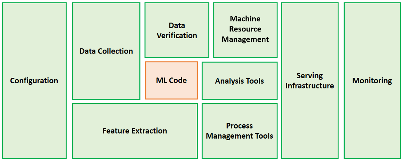
However, beyond model development, there are multiple components in a production-ready ML system that requires plenty of work.
In this comprehensive guide, we explore how to set up, train, and serve an ML system using the powerful capabilities of H2O AutoML, MLflow, Fastapi, and Streamlit to build an insurance cross-sell prediction system.
Contents
(1) Business Context(2) Tools Overview (3) Step-by-Step Implementation (4) Moving Forward
(1) Business Context
Cross-selling in insurance is the practice of promoting products that are complementary to the policies that customers already own.
Cross-selling creates a win-win situation where customers obtain comprehensive protection at a lower bundled cost. At the same time, insurers can boost revenue through enhanced policy conversions.
This project aims to make cross-selling more efficient and targeted by building an ML pipeline to identify health insurance customers interested in purchasing additional vehicle insurance.

(2) Tools Overview
H2O AutoML

H2O is an open-source, distributed, and scalable platform that enables users to easily build and productionalize ML models in enterprise environments.
One of H2O’s key features is H2O AutoML, a service that automates the ML workflow, including the automatic training and tuning of multiple models.
This automation allows teams to focus on other vital components such as data preprocessing, feature engineering, and model deployment.
MLflow

MLflow is an open-source platform for managing ML lifecycles, including experimentation, deployment, and creation of a central model registry.
The MLflow Tracking component is an API that logs and loads the parameters, code versions, and artifacts from ML model experiments.
Mlflow also comes with a _mlflow.h2o_ API module that integrates H2O AutoML runs with MLflow tracking.
FastAPI

FastAPI is a fast and highly performant web framework for building APIs in Python. It is designed to be user-friendly, intuitive, and production-ready.
The purpose of deploying our ML model as a FastAPI endpoint is to readily retrieve prediction results after parsing our test data into the API.
Streamlit

Streamlit is an open-source app framework that turns data scripts into shareable web apps within minutes. It helps create user-friendly front-end interfaces for both technical and non-technical users to interact with.
The user interface allows us to upload data to the backend pipeline via the FastAPI endpoint and then download predictions with a click of the mouse.
Virtual Environment Setup
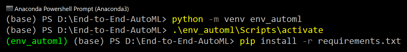
We first create a Python virtual environment using the venv module (see setup screenshot below).
After activating the virtual environment, we install the necessary packages with pip install -r [requirements.txt](https://github.com/kennethleungty/End-to-End-AutoML-Insurance/blob/main/requirements.txt) based on requirements.txt.
(3) Step-by-Step Implementation
The GitHub repo to this project can be found here, where you can find the codes to follow along.
(i) Data Acquisition and Exploration
We will be using the Health Insurance Cross-Sell Prediction data, which we can retrieve via the Kaggle API.
To use the API, go to the ‘Account’ tab (kaggle.com//account) and select ‘Create API Token‘. This action triggers the download of the kaggle.json file containing your API credentials.

We use the opendatasets package (installed with pip install opendatasets) and the credentials to retrieve the raw data:
The dataset contains 12 features describing the profiles of 380K+ health insurance policyholders. All the data have been anonymized and numericized to ensure privacy and confidentiality.
The target variable is Response, a binary measure of the customer’s interest in purchasing additional vehicle insurance (where 1 indicates positive interest).
The other variables are as follows:
- id: Unique identifier for each customer
- Gender: Gender of the customer
- Age: Age of the customer (years)
- Driving_License: Whether the customer holds a driving license (1) or not
- Region_Code: Unique code for the region that the customer is located
- Previously_Insured: Whether customer already has vehicle insurance (1) or not
- Vehicle_Age: Age of the customer’s vehicle
- Vehicle_Damage: Whether the customer got their vehicle damaged in the past (1) or not
- Annual_Premium: Sum of premiums paid by the customer in a year
- PolicySalesChannel: Anonymized code for the channel the insurance agent contacted the customer, e.g., phone, in-person
- Vintage: Number of days that the customer has been with the insurer
(ii) Data Preprocessing
Data preprocessing and feature engineering are crucial steps for any data science project. Here is a summary of the steps taken:
- Label encoding of Gender variable (1 = Female, 0 = Male)
- One-hot encoding of categorical variables
- Renaming of one-hot encoded variables for better clarity
- Min-max scaling of numerical variables
Because the focus is to showcase the setup of an end-to-end pipeline, the transformations performed are not as extensive as they can be. In real-world cases, this step deserves in-depth work as part of a data-centric approach.
(iii) H2O and MLflow Setup
Before starting model training on the processed dataset, we first initialize an H2O instance and an MLflow client.
H2O Initialization
The initialization of an H2O instance can be done with h2o.init(), after which it will connect a local H2O server at 127.0.0.1:54321.
The following printout will be displayed upon successful H2O connection.

MLflow Initialization
MLflow is initialized with client = MlflowClient(), which creates an MLflow Tracking Server client that manages our experiment runs.
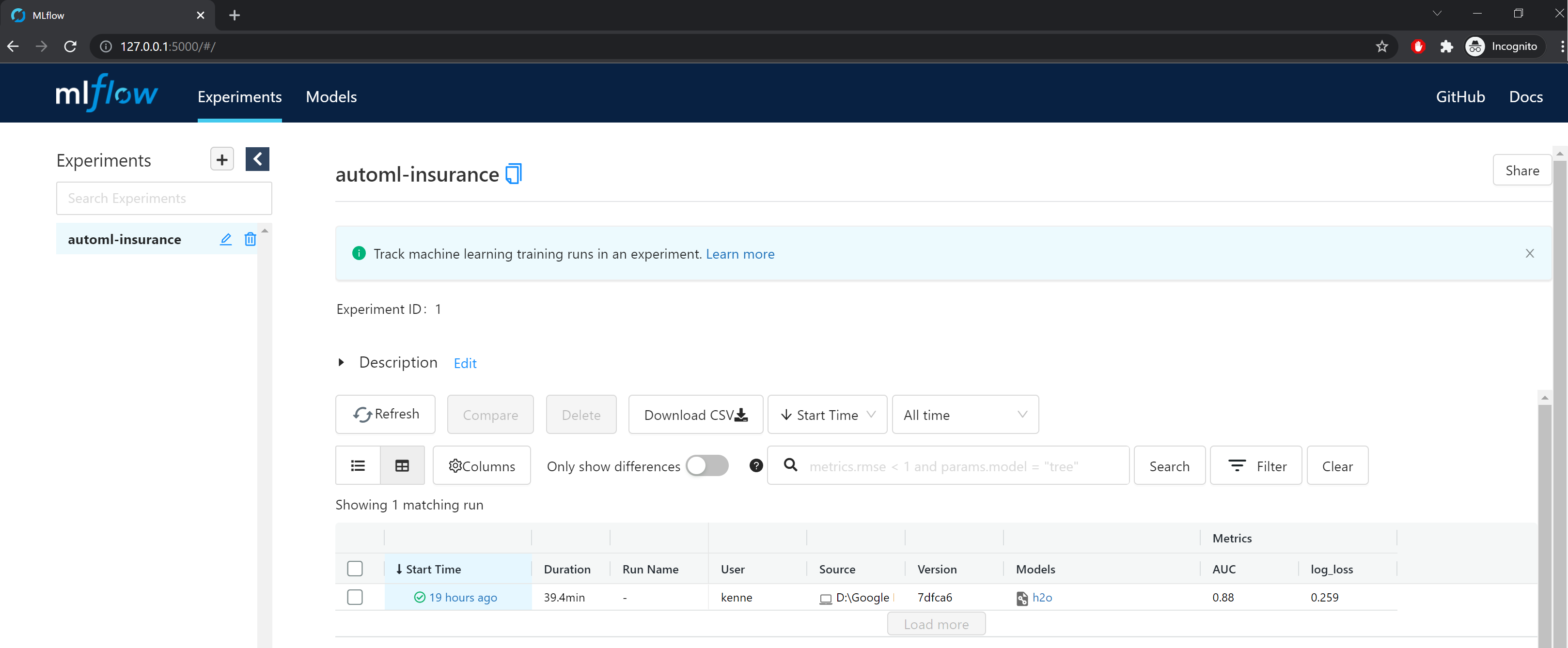
An MLflow experiment can comprise multiple ML training runs, so we start by creating and setting our first experiment (automl-insurance). The logs are recorded locally into a /mlruns subfolder by default.

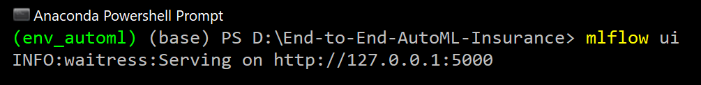
MLflow has a user interface for browsing our ML experiments. We can access the interface by running mlflow ui in command prompt (from the project directory) and then accessing the localhost URL 127.0.0.1:5000.
Beyond local file storage, there are various backend and artifact storage configurations for runs to be recorded to an SQLAlchemy compatible database or remotely to a tracking server.
(iv) H2O AutoML Training with MLflow Tracking
After importing our data as an H2O data frame, defining the target and predictor features, and setting the target variable as categorical (for binary classification), we can begin the model training setup.
H2O AutoML provides a wrapper function H2OAutoML() that performs the training of a variety of ML algorithms automatically.
As we initialize an AutoML instance (aml = H2OAutoML()), we wrap it within an MLflow context manager using mlflow.start_run() so that the model is logged inside an active MLflow run.
Here is an explanation of the AutoML instance parameters:
max_models– Maximum number of models to build in an AutoML runseed– Random seed for reproducibilitybalance_classes– Indicate whether to oversample the minority classes to balance the class distribution.sort_metric– Specifies the metric used to sort the leaderboard at the end of an AutoML runverbosity– Type of backend messages to be printed during trainingexclude_algos– Specify the algorithms to skip during model-building (I excluded GLM and DRF so that emphasis is placed on GBM algorithms)
We can then kickstart AutoML training with a single line of code:
Consider running the training on Google Colab so that you can spare your local machine from the resource-intensive training runs
(v) Log Best AutoML Model
After training is completed, we obtain a leaderboard displaying a table of candidate models. The table is sorted based on the sort_metric performance metric (log-loss) specified earlier.

The leaderboard shows that the stacked ensemble model ‘StackedEnsemble_AllModels_4’ had the best performance based on log-loss value (0.267856).
H2O’s Stacked Ensemble is a supervised ML model that finds the optimal combination of various algorithms using stacking. The stacking of algorithms delivers better predictive performance than any of the constituent learning algorithms.
The next thing to do is log the best AutoML model (aka AutoML leader). As part of logging, we also import the mlflow.h2o module. There are three aspects of the AutoML model we want to log:
- Metrics (e.g., log-loss, AUC)
- Model artifacts
-
Leaderboard (saved as CSV file within artifacts folder)
You can execute AutoML training with the train.py script. This can be done with
python train.py - -target 'Response'in command prompt.
H2O also offers model explainability for you to explain the inner workings of the models to technical and business stakeholders.
(vi) Generate and Evaluate Predictions
After numerous runs of an experiment (or different experiments), we want to select the best model for model inference.
We can use mlflow.search_runs() to find the best-performing model, mlflow.h2o.load_model() to load the H2O model, and .predict() to generate predictions.
How does the AutoML model fare against a baseline model like XGBoost with RandomizedSearchCV? Here are the results after evaluating their predictions:

The AutoML model outperforms the baseline by a slight margin. This better performance is a testament to the capabilities of AutoML in delivering performant models with speed and ease.
Do check out the notebooks detailing the training and prediction of both models:
(vii) FastAPI Setup
Now that we have selected our best model, it is time to deploy it as a FastAPI endpoint. The goal is to create a backend server where our model is loaded and served to make real-time predictions through HTTP requests.
Inside a new Python script main.py , we create a FastAPI instance with app = FastAPI(), and then set a path operation @app.post("/predict")to generate and return predictions.
We also include the codes for H2O and MLflow initialization and the codes for model inference from Step vi.
The model inference code from Step vi is meant to retrieve the best model out of all the experiments, but you can alter the ID parameters so that a model of a specific experiment run is used.
The path operator will receive the test data as a bytes file object, so we use BytesIO as part of the data conversion into H2O frame.
Finally, we want a JSON output that contains the model predictions. The output can be returned as JSON files using JSONResponse from fastapi.responses.
You can find the complete FastAPI code in the main.py script.
The final part is to activate our FastAPI endpoint by running the uvicorn server (from the backendsubdirectory where the script is stored) with the following command:
uvicorn main:app --host 0.0.0.0 --port 8000
The FastAPI endpoint will be served in the local machine, and we can access the API interface at 127.0.0.1:8000/docs (or localhost:8000/docs)
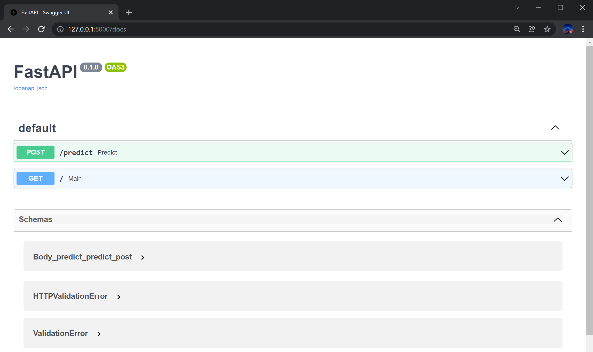
We see that our /predict path operator is present on the /docs page of the FastAPI interface, indicating that the API is ready to receive data via POST requests.
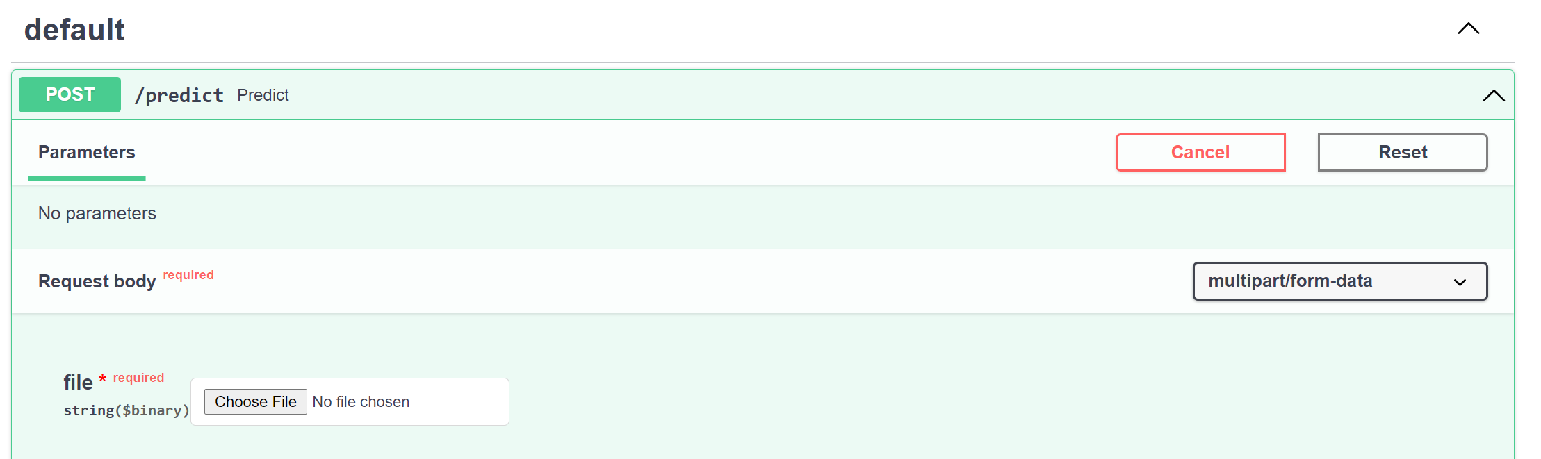
As we click into the POST section, we see that the API has been correctly set up to receive binary files, e.g., CSV files.
At this point, we can already retrieve predictions by using the requests module and several lines of Python codes in a Jupyter notebook.
However, a great way to bring this system up a notch is to build a web app with a graphical user interface for users to upload data and download predictions with just a few clicks of the mouse.
(viii) Setup and Build Streamlit Web App
Streamlit provides a simple framework to build web apps, enabling data teams to showcase their ML products readily.
The objective of the web app is for users to upload data files, run model inference, and then download the predictions as a JSON file, all done without writing any code.
We create a new script app.py to house the Streamlit codes for the following key components:
- File uploader for the selection of the CSV or Excel test dataset file
- Read file as Pandas data frame and display first five rows (for sanity check)
- Convert data frame into a BytesIO file object
- Display a ‘Start Prediction’ button which, when clicked, will parse the BytesIO object into the FastAPI endpoint via
requests.post() - Upon completing model inference, a ‘Download‘ button appears for users to download the predictions as a JSON file.
As part of model inference, we also include the definition of our endpoint – [http://localhost:8000/predict](http://localhost:8000/predict.).
In the GitHub repo, you can find the complete Streamlit code in the app.py script.
(ix) Initialize FastAPI and Streamlit Servers
By now, all our Python scripts for FastAPI and Streamlit functions are ready. We next initialize both servers in the command prompt.
(1) If your uvicorn server (for FastAPI) is still running from Step vii, you can leave it as such. Otherwise, open a new command prompt, go to the /backend subdirectory containing the main.py script, and enter:
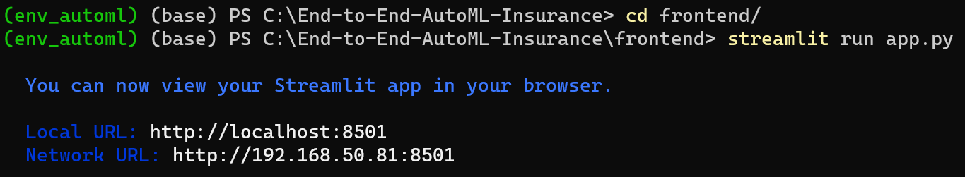
uvicorn main:app --host 0.0.0.0 --port 8000(2) Open another separate command prompt and initialize the Streamlit server (from the frontend folder containing the script) with: streamlit run app.py
(x) Run Prediction and Download Results
With the FastAPI and Streamlit servers up and running, it is time to access our Streamlit web app by heading to http://localhost:8501.
The following gif illustrates the web app’s simplicity, from data upload to prediction download.
Note: The file used for the demo prediction is data/processed/test.csv
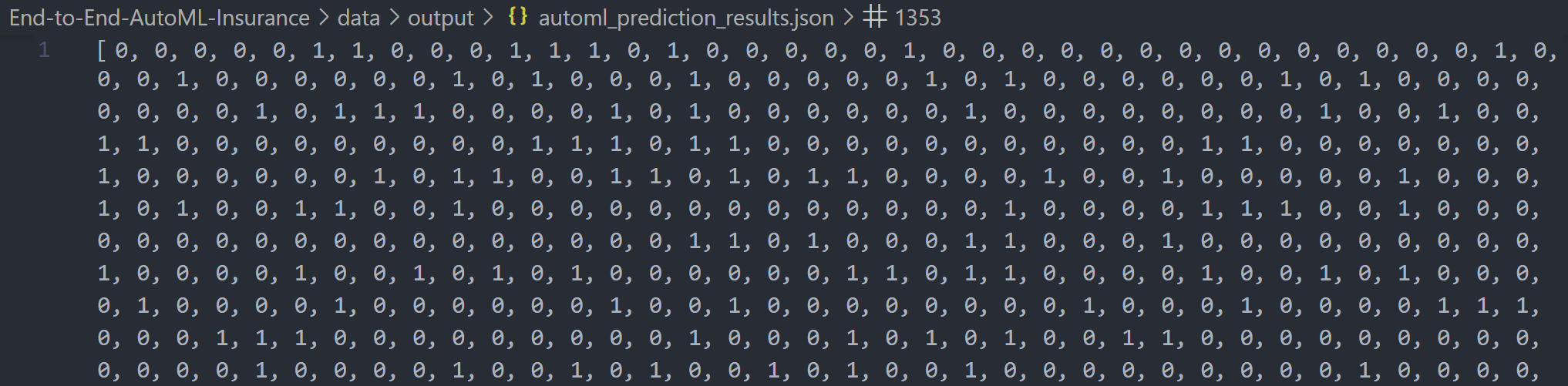
Here is a snapshot of the JSON output containing the predictions (1 or 0) for each customer:
(4) Moving Forward
Let’s recap what we have done. We first conducted H2O AutoML training and MLflow tracking to develop various ML models.
We then retrieved the best-performing model and deployed it as an endpoint using FastAPI. Finally, we created a Streamlit web app to upload test set data and download the model predictions easily.
You can find the project GitHub repo here.
While extensive work has been done so far in successfully building our end-to-end ML pipeline, there are a couple of steps ahead of us to complete the whole picture. These tasks include:
- Dockerization of this entire ML application and deployment on cloud
- Pipeline orchestration in Docker (e.g., Airflow, Kedro)
And here is the sequel to this article where we used Docker to containerize this entire pipeline:
How to Dockerize Machine Learning Applications Built with H2O, MLflow, FastAPI, and Streamlit
Before You Go
I welcome you to join me on a data science learning journey! Follow my Medium page and GitHub to stay in the loop of more exciting data science content. Meanwhile, have fun building end-to-end AutoML solutions!
Key Learning Points from MLOps Specialization – Course 2


