
Large Language Models (LLMs) have taken the world by storm. Over the last year we have witnessed a massive leap in what they can do, going from quite narrow and restricted applications to now engaging in fluent, multi-turn conversations.
Isn’t it amazing how these models have shifted from extractive summarization—copying the source verbatim—to now providing abstractive summarizations? They are now completely re-writing the summary to match the reader’s style preference and the reader’s existing knowledge. What’s even more astonishing is that these new models can not only generate new code, but explain your existing code. Fascinating.
Frequently these large models are so powerful that they even yield impressive results when queried in a zero-shot or few-shot manner. Although this allows for rapid experimentation and seeing results immediately, for many tasks this is often followed by finetuning a model to achieve the best performance and efficiency. However, finetuning every single one of their billions of parameters becomes impractical inefficient. Moreover, given the size of the models, do we even have enough labeled data to train such a massive model without overfitting?
Parameter Efficient Finetuning (Peft) to the rescue: You can now achieve great performance while only tuning a small fraction of the weights. Not having to tune billions of parameters across multiple machines, makes the whole process of finetuning more practical and economically viable again. Using PEFT and quantization allows large models with billions of parameters to be finetuned on a single GPU.
This mini-series is for experienced ML practitioners who want to explore PEFT and specifically LoRA [2]:
- In Article One we explore the motivation for parameter efficient finetuning (PEFT). We review why and how finetuning works, what aspects of our existing practices can be retained, generalized and applied in a refined fashion. We’ll get hands-on and implement the essentials from scratch to create an intuitive understanding and to illustrate the simplicity of the method we chose to explore, LoRA.
- In Article Two we now dive into finding good hyperparameter values, i.e. we review the relevant design decisions when applying LoRA. Along the way we establish baselines for performance comparisons and then review the components that we can adapt using LoRA, what their impact is and how we can appropriately size them.
- Based on a trained and tuned model for a single task, in Article Three we now extend our view to tuning multiple tasks. Also, what about deployment? How can we use the relative small footprint of the adapters we trained for a single task and implement a hot-swapping mechanism to use a single model endpoint to do inference for multiple tasks.
- Over the course of the first three articles, we have developed an intuitive grasp of training, tuning and deploying using PEFT. Transitioning into Article Four we’ll become very practical. We’ll step away from our educational model, asking "What have we learned so far and how do we apply this to a real world scenario?" We then use the established implementation by Hugging Face to meet our goals. This will include using QLoRA, that marries LoRA and quantization for efficient GPU memory usage.
Ready to dive in? For today, let’s start with why this all works.
On The Effectiveness Of Pre-Training and Finetuning
In their work Aghajanyan et al [1] showed two interesting observations about how the neural network layers change during pre-training, making it easier to do finetuning. This is broadly applicable, not just for a specific finetuning task.
Specifically they show that pre-training minimizes the intrinsic dimensionality (ID) of the representations. The following two figures – taken from their work – illustrate the effect:


Rather than finetuning all parameters, the authors trained the respective models with a smaller, randomly selected, subset of parameters. The number of parameters was chosen to match 90% of the performance of full finetuning. This dimensionality, required to achieve 90% performance, is denoted as d90 on the two y-axes in the figure above.
The first figure shows that with an increase in pre-training duration, on the x-axis, d90 goes down, i.e. the number of parameters needed in the following finetuning to achieve 90% of the full finetuning performance decreases. Which in itself shows the effectiveness of pre-training as a way to compress knowledge.
In the second figure we can also see that with increased capacity the number of parameters needed to achieve d90 in the finetuned model goes down as well. How interesting. It indicates that a larger model can learn a better representation of the training data—the world the model sees—and creates hierarchical features that are easy to use in any downstream task.
One specific example the authors point out is that d90 for RoBERTa Large (354M) is about 207 parameters. Bam!
Please find that example in the diagram above and then also check that the smaller RoBERTa Base (123M) needs more parameters to achieve 90% performance, here 896. Interesting.
From discussions I had on this topic I learned that there are a few things worth pointing out explicitly:
- We leverage the effect of ID during finetuning, but the graphs and numbers above are all about the pre-training. We just use the finetuning numbers to make the resulting downstream impact more tangible.
- Using a larger model not only results in a lower ID relative to their size, but also absolutely. We will see a similar effect when moving to PEFT.
In [1] you will find the above illustrations as figure 2, figure 3 and the cited results are taken from table 1.
In conclusion, we can see that the learned representations during pre-training compress the knowledge that the model learned and make it easier to finetune a downstream model using these more semantic representations. We’ll built on top of that with PEFT. Only, instead of selecting the parameters to tune randomly and to aim for 90% performance, we will use a more directed approach to select which parameters to train and aim to almost match the performance of the full finetuning. Exciting!
What to Tune?
We have established that we can work with a very small number of parameters. But which ones? Where in the model? We’ll go into much more details in the next article. But to get our thinking started and to frame our problem, let’s reflect on two general approaches for now:

Based on the task: When using finetuning, we want to retain the knowledge from the pre-training and to avoid "catastrophic forgetting". We recognize that the downstream task-specific learnings should happen in the task head, here the classifier, of the finetuned model and in the immediate layers below the head (depicted in green), while in the lower layers and embeddings we want to retain the general knowledge we learned about the use of language (in red). Frequently we guide the model then with per-layer learning rates, or even completely freezing the lower layers.
This is all based on our understanding on where we expect the model to learn the essential knowledge for our downstream task, and where existing knowledge from the pre-training should be retained.

Based on the architecture: In contrast, we can also review the components of our architecture, their parameters and their possible impact. In the illustration above you see for example LayerNorm and Biases, which are of low capacity, but spread out all over the model. These are in central positions to impact the model, but have relatively few parameters.
On the other hand, we have the parameters from the embeddings. These are not close to the task, but close to the inputs however. And we have a lot of parameters in the embeddings. So if we want to be efficient they would not be our first choice for any kind of finetuning, including PEFT.
And last, not least, we have the large linear modules that come with the transformers architecture, namely the attention vectors and the feed forward layers. These have a large number of parameters and we can decide on which layer to adapt them.
We’ll revisit selecting the right parameters in the next article in more detail. For this article, no matter how we want to slice and dice the problem, we will end up with groups of parameters that we want to tune. For the rest of this article it will be some linear modules.
Using Adapters to Become More Efficient
Instead of tuning a whole linear module with all of its parameters we want to be more efficient. The approach we use is injecting adapters. These new modules are relatively small and will be placed after the module we want to adapt. The adapters can modify the output of the linear modules, i.e. they can refine the pre-trained outputs in a way that is beneficial to the downstream-task.

But there is a problem with this approach. Can you spot it? It’s about the relative sizes of the module to be adapted and the adapter. If you look at the illustration below, you see the GPU memory. For efficiency we size our model so that it can fit as tightly as possible into the available GPU memory. This is particularly easy with the Transformer architecture due to each layer being of the same width, and even the down projected heads add up to the full width again. Hence we can pick a batch-size based on the uniform width of the Transformer’s components.
But if we now inject very small adapters after larger linear layers, we have a problem. Our memory use becomes inefficient as can be seen in the illustration below.
The batch-size fits the width of the Linear layer, but now we have a much smaller adapter. Therefore most of the GPU has to wait for the small adapter to be executed. This lowers the GPU utilization. And it’s worse than it looks in the illustration, keeping in mind that the area of the adapter in the diagram is supposed to be around 1%, while in the illustration it looks closer to 20%.

One way to deal with this is to parallelize the adaptation and just connect them with an addition, allowing both paths to contribute to the output. This way we don’t have a memory bottleneck anymore and can execute both the original linear module and the adapter in parallel, avoiding the gaps we saw before.
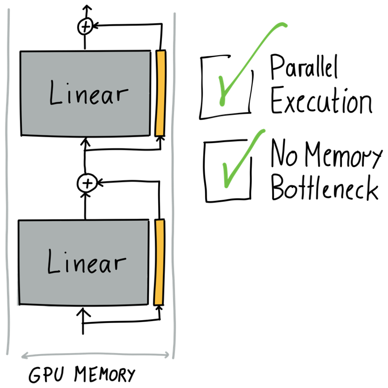
But even the execution in parallel is an additional burden compared to having no adapter at all. This is true for training, but would even be true for inference. That’s not ideal. Also, how big should such an adapter be?

We will deal with the inefficiency during inference in the third article. Sneak peek: It’s going to be fine – we will merge the module’s weights with the product of the low rank matrices. Back to this article – let’s tackle the adapter size.
Low Ranking Matrices As Adapters
Let’s zoom in.
Below, you see the original linear module in grey on the left and the adapter in orange on the right. To make them compatible, the inputs and outputs must match, so that we can call them in parallel with the same input and then add up the outputs, similar to using a residual connection. Hence the input and output dimensions on both sides must match.
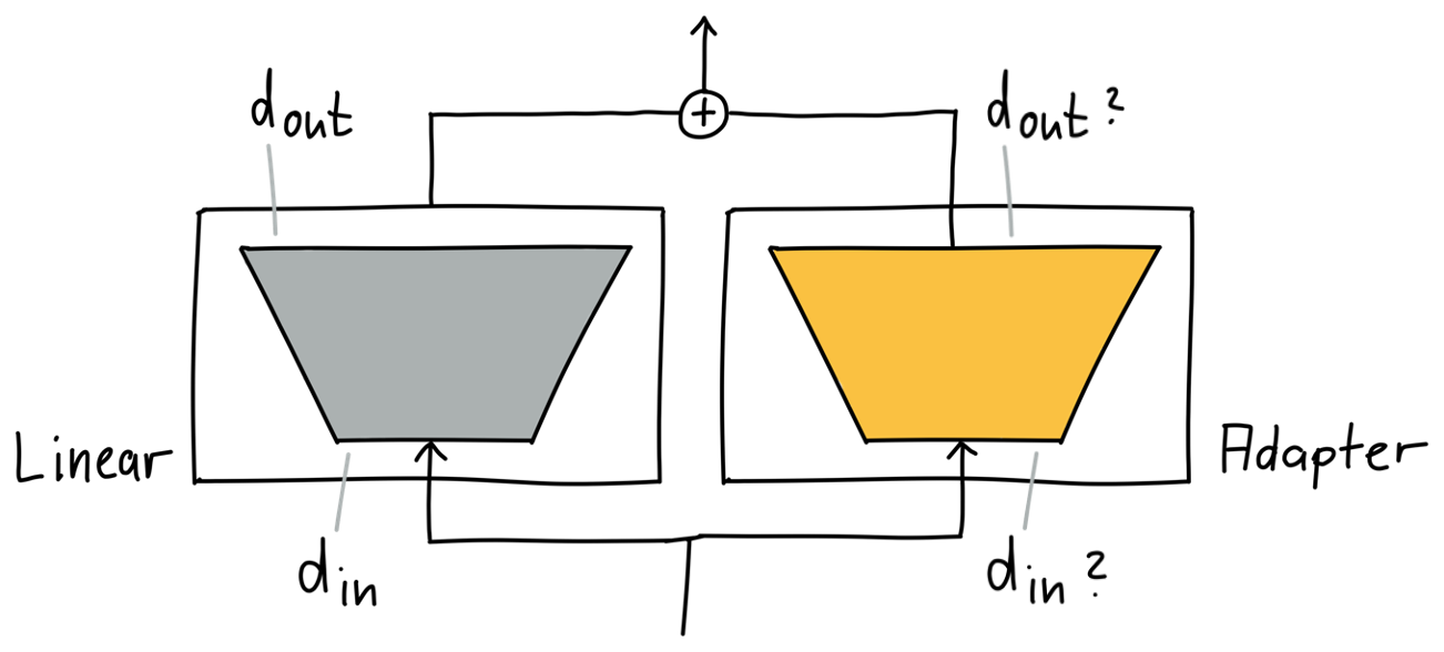
The linear module and the adapter translate to two matrices. And given their matching dimensions, mechanically, we have compatibility now. But as the adapter is as big as the the module we are adapting, we did not become more efficient. We need to have an adapter, that is small and compatible.
The product of two low rank matrices fits our requirements:

The large matrix is decomposed in two low rank matrices. But the matrices themselves are much smaller, d_in x r and r x d_out, especially as r is much smaller as d_in and d_out. We typically look at numbers like 1, 2, 4, 16 for r, while d_in and d_out are like 768, 1024, 3072, 4096.
Let’s put this all together:

We can see that we have a singlex as input. x is then multiplied with the original weights, W0. W0 are the pre-trained weights. And x is multiplied with A and B, and eventually both results are added and form the adjusted output, here named x'.
There are different adapter implementations, but in LoRA we make this an optimization problem and both low rank matrices A and B are learned for the specific downstream task. Learning those fewer parameters is then more efficient than learning all parameters in W0.
Initialization
Let’s go on a quick tangent. How would you initialize A and B? If you initialize it randomly, consider what would happen in the beginning of the training?
In each forward pass we would add random noise to the output of an adapted module and we would have to wait for the optimizer to step-by-step correct the wrong initialization, leading to instabilities at the beginning of the finetuning.
To mitigate we typically use lower learning rates, smaller initialization values or warm up periods where we limit the effect that these wrong parameters can have, so that we do not destabilize the weights too much. In the LLAMA adapter [3] paper the authors introduce zero gating: They start the value of an adapter’s gate—to be multiplied with the actual weights—with 0 and increase its value over the course of the training.
An alternative approach would be to initialize Aand B with 0. But then you would not be able to break symmetry and in the learning process all parameters may be treated as one parameter.
What LoRA actually does is quite elegant. One matrix, A, is initialized randomly, while the other matrix, B, is initialized with 0. Hence the product of the two matrices is 0, but still each parameter can be differentiated individually during backpropagation. Starting with 0 means that the inductive bias is to do nothing, unless changing the weights will lead to a loss reduction. So there will be no instabilities at the beginning of the training. Nice!

How Could That Look like in Code?
Let’s check out some code excerpts for our small, illustrative example. You find the full code in the accompanying notebook and a more complete implementation that we use in the following articles is in the same repository.
Let’s start with how we setup an adapter. We pass in a reference to the module to be adapted, which we now call the adaptee. We store a reference to its original forward method and let the adaptee‘s forward method now point to the adapter’s forward method’s implementation.
class LoRAAdapter(nn.Module):
    def __init__(self,
                 adaptee, # <- module to be adapted
                 r):
        super().__init__()

        self.r = r
        self.adaptee = adaptee

        # Store a pointer to the original forward implementation
        # of the module to be adapted.
        # Then point its forward method to this adapter module.
        self.orig_forward = adaptee.forward
        adaptee.forward = self.forward
        [..]
Now that we have setup the mechanics of the integration, we also initialize the parameters of our low rank matrices. Recognize that we initialize one matrix with 0 and one randomly:
        [..]
        # Adding the weight matrices directly to the adaptee,
        # which makes it more practical to report the parameters,
        # and to remove it later.
        adaptee.lora_A = (nn.Parameter(torch.randn(adaptee.in_features, r)/
                          math.sqrt(adaptee.in_features)))
        adaptee.lora_B = nn.Parameter(torch.zeros(r, adaptee.out_features))
And finally, still part of the LoRAAdapter class, we have our forward method that first calls the adaptee‘s forward method with our input x. That is the original path executed in the original module. But we then also add that result to that from our adapted branch, where we matrix multiply the input x with A and B.
def forward(self, x, *args, **kwargs):
  return (
    self.orig_forward(x, *args, **kwargs) +
    x @ self.adaptee.lora_A @ self.adaptee.lora_B
  )
This simplicity looks elegant to my eye.
There are more details that could be interesting, but are best explained alongside code. You find these in the accompanying notebook:
- How to first freeze the whole model
- How to then unfreeze the classifier. As it is specific to our downstream task and we completely train it.
- How to add adapters; which are all active, not frozen.
- Reviewing how the dimensions of the module’s matrix relate to the two lower rank matrices
AandB. - How much smaller is the number of parameters when using a small value for
r?
A small excerpt below shows how the parameters of the original module output.dense are not trained (marked with a 0 ), but its LoRA matrices are trainable (marked with a 1) and, of course, the overall classifier of the model (also marked as trainable with a 1):
[..]
roberta.encoder.layer.11.attention.output.LayerNorm.bias       0         768
roberta.encoder.layer.11.intermediate.dense.weight             0     2359296
roberta.encoder.layer.11.intermediate.dense.bias               0        3072
roberta.encoder.layer.11.output.dense.weight                   0     2359296
roberta.encoder.layer.11.output.dense.bias                     0         768
roberta.encoder.layer.11.output.dense.lora_A                   1       12288
roberta.encoder.layer.11.output.dense.lora_B                   1        3072
roberta.encoder.layer.11.output.LayerNorm.weight               0         768
roberta.encoder.layer.11.output.LayerNorm.bias                 0         768
classifier.dense.weight                                        1      589824
classifier.dense.bias                                          1         768
classifier.out_proj.weight                                     1        1536
classifier.out_proj.bias                                       1           2
[..]
Total parameters: 124,978,946, thereof learnable: 923,906 (0.7392%)
Check out the notebook for more.
Take It for a Spin?
Further, you will see some tests in the notebook that show that the whole setup works mechanically.
But then we run our first experiment and submit the Training Jobs to SageMaker. We do a full finetuning on the original model and then a training with LoRA enabled as described here.
For our test, we train RoBERTa Large [4] on the sst-2 dataset [5] with r=2 adapting the query and output parameters on all layers. We use 5e-5 and 4e-4 as learning rates for the full-finetuning and the LoRA finetuning.
That’s the result (more in the notebook):
full-finetuning accuracy: 0.944
lora-finetuning accuracy: 0.933
So that’s … great, not so great? What is it? First, it clearly shows that the whole setup works on a mechanical level – that’s great. And an accuracy over 90% shows that it is working well.
But how well? What do we compare these numbers to? And how representative are these two individual training runs? Were we just lucky or unlucky? The LoRA numbers are better than the traditional approach? Isn’t that strange. How well did we tune the traditional approach?
None of the above results are reliable. We don’t know if using our hyperparameters on a second run would produce similar results. Also, we used hyperparameters selected with a semi-educated guess.
There is, of course, a better way. And so in the next article we will apply a more serious approach to selecting hyperparameters and will be evaluating the performance more systematically:
- Establish baselines for comparisons
- Search good hyperparameters for both the baselines and the experiments
- Most importantly: Deepen our understanding of the LoRA method and the impact of design decisions, aligning our intuitions in a data-driven fashion
Until then, I hope you had fun reading this article.
Thanks to Constantin Gonzalez, Ümit Yoldas, Valerio Perrone and Elina Lesyk for providing invaluable feedback during the writing of this article.
All images by the author unless otherwise noted.


