
In a classical time series forecasting task, the first standard decision when modeling involves the adoption of statistical methods or other pure Machine Learning models, including tree-based algorithms or deep learning techniques. The choice is strongly related to the problem we are carrying out but in general: statistical techniques are adequate when we face an autoregressive problem when the future is related only to the past; while machine learning models are suitable for more complex situations when it’s also possible to combine variegated data sources.
In this post, I try to combine the ability of the statistical method to learn from experience with the generalization of deep learning techniques. Our task is a multivariate time series forecasting problem, so we use the multivariate extension of ARIMA, known as VAR, and a simple LSTM structure. We don’t produce an ensemble model; we use the ability of VAR to filter and study history and provide benefit to our neural network in predicting the future.
Our workflow can be summarized as follow:
- Estimate a VAR properly on our training data;
- Extract what VAR has learned and use it to improve the training process of an LSTM model performing a two-step training.
We’ll see that our results aren’t obvious because, following this procedure, we have to fight the problem of Catastrophic Forgetting.
THE DATA
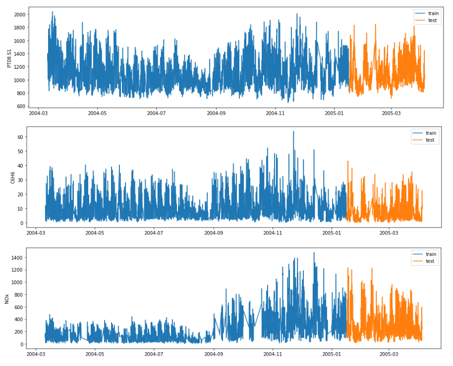
The data for our experiment contains hourly averaged responses from metal oxide chemical sensors embedded in an Air Quality Multisensor Device, located on the field in a significantly polluted area of an Italian city. Data were recorded for one year and contains ground truth hourly averaged concentrations for CO, Non-Metanic Hydrocarbons, Benzene, Total Nitrogen Oxides (NOx), and Nitrogen Dioxide (NO2). Also, external variables are provided like weather conditions. A good amount of NaNs are present, so a linear interpolation is required before proceeding (series with more than 50% of NaNs in train data are excluded).
VAR MODELING
With ARIMA we are using the past values of every variable to make the predictions for the future. When we have multiple time series at our disposal, we can also extract information from their relationships, in this way VAR is a multivariate generalization of ARIMA because it understands and uses the relationship between several inputs. This is useful for describing the dynamic behavior of the data and also provides better forecasting results.
To correctly develop a VAR model, the same classical assumptions encountered when fitting an ARIMA, have to be satisfied. We need to grant stationarity and leverage autocorrelation behaviors. These prerequisites enable us to develop a stable model. All our time series are stationary in mean and show a daily and weekly pattern.

After these preliminary checks, we are ready to fit our VAR. The choice of the perfect lag order is made automatically with the AIC/BIC criterion. We operate the selection with the AIC: all we need to do is recursively fitting our model changing the lag order and annotate the AIC score (the lowest the better). This process can be carried out considering only our train data. In our case, 27 is the best lag order.

COMBINE VAR AND LSTM
Now our scope is to use our fitted VAR to improve the training of our neural network. The VAR has learned the internal behavior of our multivariate data source adjusting the insane values, correcting the anomalous trends, and reconstructing properly the NaNs. All these pieces of information are stored in the fitted values, they are a smoothed version of the original data which have been manipulated by the model during the training procedure. In other words, we can see these values as a kind of augmented data source of the original train.
Our strategy involves applying a two-step training procedure. We start feeding our LSTM autoencoder, using the fitted values produced by VAR, for multi-step ahead forecasts of all the series at our disposal (multivariate output). Then we conclude the training with the raw data, in our case they are the same data we used before to fit the VAR. With our neural network, we can also combine external data sources, for example, the weather conditions or some time attributes like weekdays, hours, and months that we cyclically encode.
We hope that our neural network can learn from two different but similar data sources and perform better on our test data. Our approach sounds great but this is not a ‘free lunch’. When performing multiple-step training we have to take care of the Catastrophic Forgetting problem. Catastrophic forgetting is a problem faced by many models and algorithms. When trained on one task, then trained on a second task, many machine learning models "forget" how to perform the first task. This is widely believed to be a serious problem for Neural Networks.
To avoid this tedious problem, the structure of the entire network has to be properly tuned to provide a benefit in performance terms. From these observations, we preserve a final part of our previous training as validation.
Technically speaking the network is very simple. It’s constituted by a seq2seq LSTM autoencoder which predicts the available sensors N steps ahead in the future. The training procedure is carried out using keras-hypetune. This framework provides hyperparameter optimization of the neural network structures in a very intuitive way. This is done for all three training involved (the fit on VAR fitted values, the fine-tuning fit with the raw data and the standard fit directly on the raw data).
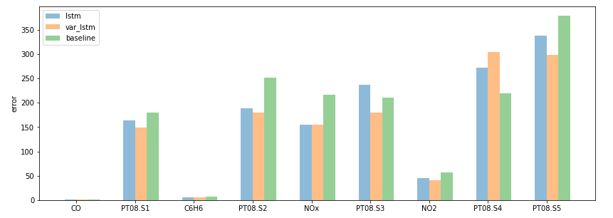
In the end, we can compare the model trained on the fitted values of the VAR plus the original data and the same structure trained only on the original training data. The errors, in most cases, are lower when we perform the two training steps. We report also the performance obtain with a baseline, composed of a simple repetition of the last available observations. This procedure is a good practice to verify if the predictions are not the present values repeated, i.e. not a useful prediction.
SUMMARY
In this post, we tried to use the information learned by a VAR model, for a multivariate time series task, to improve the performance of a recurrent neural network trained to predict the future. We operated a two-step training procedure, fighting the problem of Catastrophic Forgetting and achieving an improvement in the overall performance.
Keep in touch: Linkedin
REFERENCES
An Empirical Investigation of Catastrophic Forgetting in Gradient-Based Neural Networks: Ian J. Goodfellow, Mehdi Mirza, Da Xiao, Aaron Courville, Yoshua Bengio


