Recurrent Neural Networks (RNNs) are regular feedforward neural network variants that handle sequence-based data like time series and natural language.
They achieve this by adding a "recurrent" neuron that allows information to be fed through from past inputs and outputs to the next step. The diagram below depicts a traditional RNN:
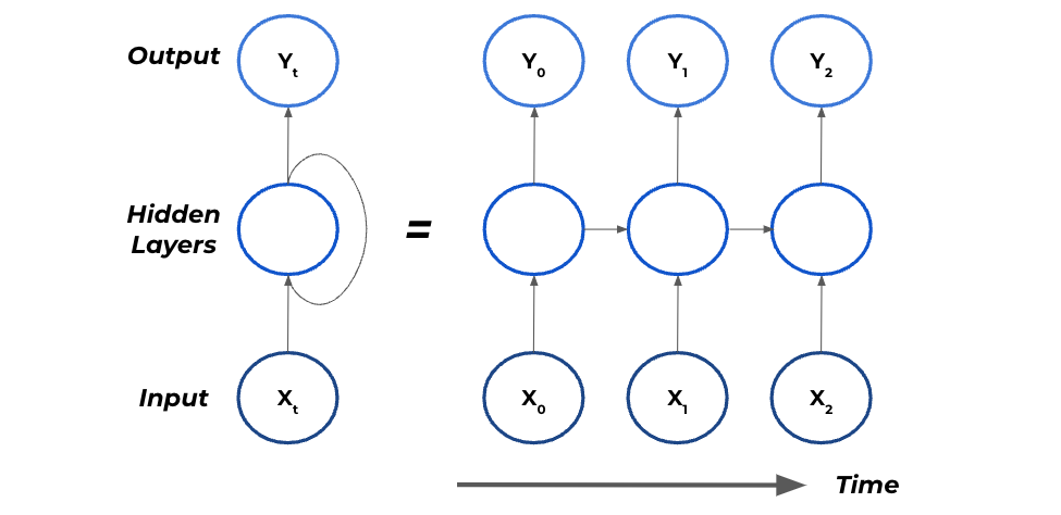
On the left side is a recurrent neuron, and on the right-hand side is the recurrent neuron unrolled through time. Notice __ how the previous executions are passed on to the subsequent calculations.
This adds some inherent "memory" in the system that aids the model in picking up historical patterns that happened previously in time.
When predicting _Y_1, the recurrent neuron uses the inputs of X_1 and the output from the previous time step, Y_0. This means that Y_0′s influence on Y_1 is direct, and it also indirectly influences Y_2._
If you want a complete introduction to RNNs and some worked examples, check out my previous post.
Recurrent Neural Networks – An Introduction To Sequence Modelling
However, in this article we are going to go over exactly how RNNs learn using something called Backpropagation through time (BPTT)!
What Is Backpropagation?
Before diving into Bptt, its worth recapping over normal backpropagation. Backpropagation is the algorithm used to train the regular feed-forward neural networks.
The essence of backpropagation is to adjust each parameter in the neural network based on the loss function, aiming to minimise the error. This adjustment is made using partial derivatives and the chain rule.
Let me show you a straightforward example through compute graphs, which resemble neural networks very well.
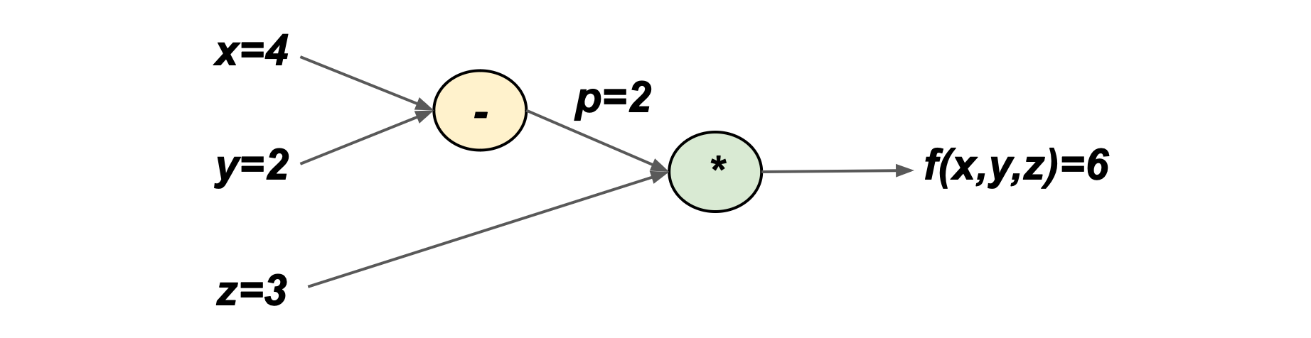
Consider the following function:

We can plot it as a compute graph, which is just a way of visualising the function:

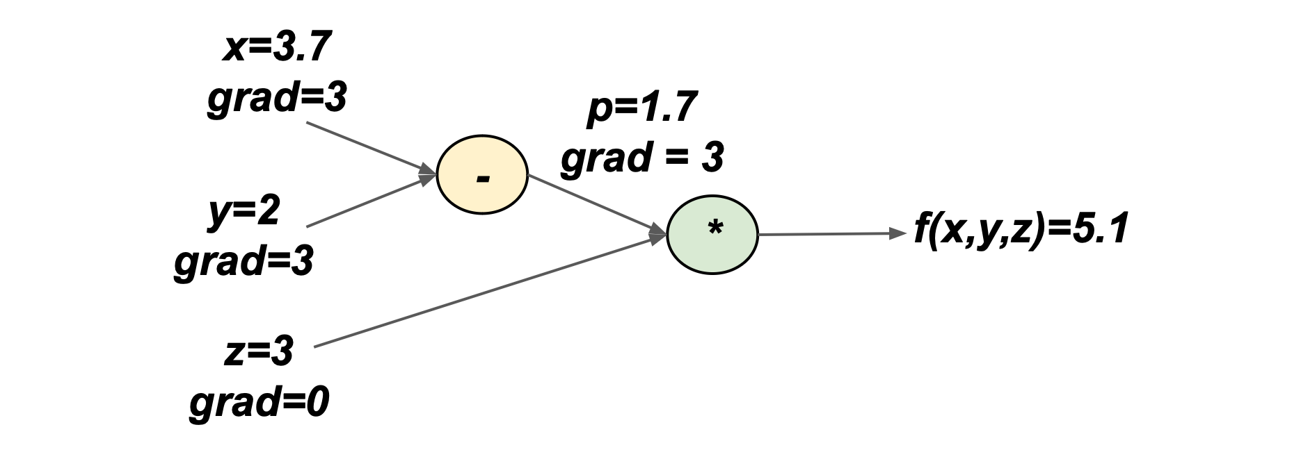
Let’s now plug in some random numbers:
The minimum of f(x,y,z) can be calculated using calculus. Notably, we need to know the partial derivative of f(x,y,z) with respect to all three of its variables: x, y, and z.
We can start by calculating the partial derivatives for p=x-y and f=pz:

But, how do we get?

Well, we use the _chain rule! This is an example for x_:

By combining different partial derivatives, we can get our desired expression. So, for the example above:

The gradient of the output, f, with respect to x is z. This makes sense as z is the only value we multiply x.
Repeating for y and z:

We can write these gradients and their corresponding values on the compute graph:
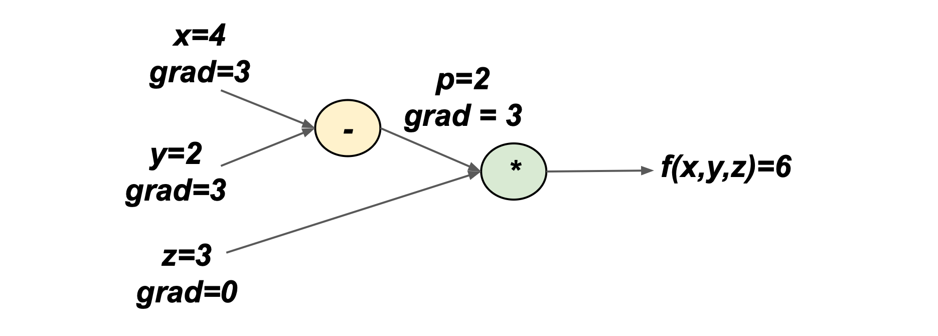
Gradient descent works by updating the values (x,y,z) by a small amount in the opposite direction of the gradient. The goal of gradient descent is to try and minimise the output function. For example, for x:

Where h is called the learning rate, it decides how much the parameter will get updated. For this case, let’s define h=0.1, so x=3.7.
What is the output now?
The output got smaller, in other words, it’s getting minimised!
I hope this gives you some intuition about how backpropagation works. It’s basically just gradient descent, but it uses the chain rule to pass on upstream gradients.
I have a full article on backpropagation, in case you want to read further.
What Is Backpropagation Through Time?
Overview
So, we have just seen that backpropagation is just gradient descent, but we are propagating the error (derivatives) backwards at each network layer.
BPTT extends this definition by carrying backpropagation at each point in time. Let’s walk through an example.
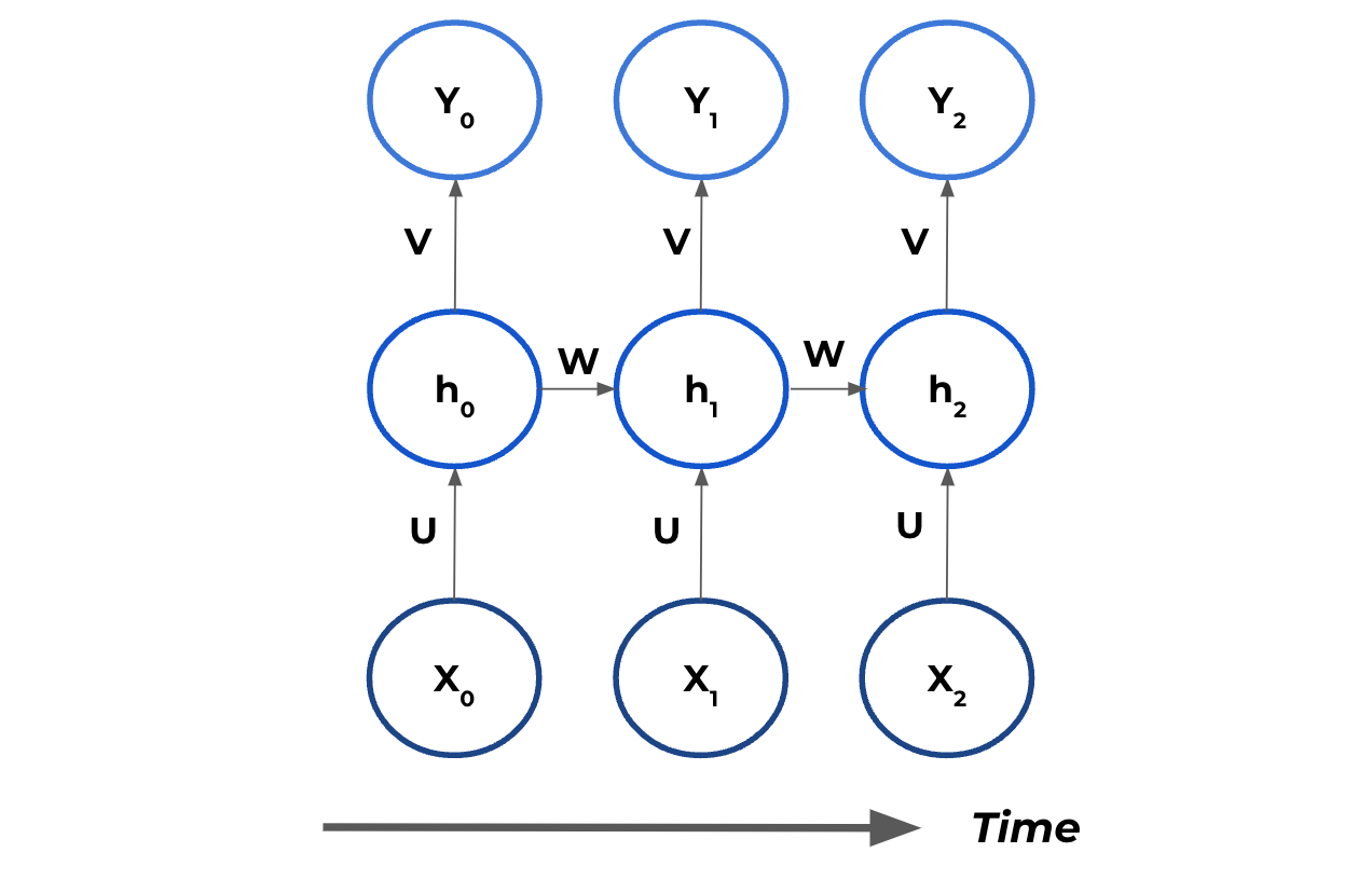
In this diagram:
- Y is the output vectors
- X are the input vectors for the features
- h are the hidden states
- V is the weighted matrix for the output
- U is the weighted matrix for the input
- W is the weighted matrix for the hidden states
I have omitted the bias terms for simplicity.
For any time t the following is the computed output:

Here we have σ as an activation function, typically tanh or sigmoid.
Let’s say our loss function is the mean squared error:

Where _A_t_ is the actual value that we want our prediction to equal.
Backpropagation Through Time
Now, we are in a position to start doing BPTT after this problem has been set up.
Remember, the goal of backpropagation is to adjust the weights and parameters of our model to minimise the error. This is done by taking the partial derivative of the weights and parameters with respect to the error.
Let’s start by calculating the updates for time step 3.
For the V weighted matrix:

This one is pretty straightforward, _E_3 is a function of Y_3, so we ** differentiate E_3 with respect to Y_3 and Y_3 with respect to V.**_ Nothing too complicated happening here.
For the W weighted matrix:

Now it’s getting a bit fancy!
The first term in the expression is relatively straightforward_. E_3 is a function of Y_3, Y_3 is a function of h_3, h_3 is an element in W. This is the same process we saw for the V_ matrix.
However, we can’t just stop there as matrix W is also used in previous steps for _h_2 and h_1_, so we have to differentiate with respect to those past steps.
We need to consider the effect of W across all time steps since the state _h_3_ depends on previous states in the RNN.
For the U weighted matrix:

The error with respect to the U matrix is very similar to that for W, with the difference that we differentiate the hidden states h with respect to U.
Remember, the hidden state is a composite function of the previous hidden state and the new input.
Generalised Formula
BPTT can be generalised as follows:

Where J is an arbitrary weight matrix in the RNN, which will be either U, W or V.
The total error (loss) of an RNN is the sum of the errors, _E_t_, at every time stamp:

And, that’s pretty all there is to training an RNN! However, there is one problem …
Exploding & Vanishing Gradient Problem
Overview
One of the significant problems with RNNs is the vanishing and exploding gradient problem. This is because when carrying out BPTT, we are essentially unrolling the network T number of time steps. The network effectively has T layers.
There are often quite a significant number of timestamps, so the unrolled network is usually very deep. As the gradient is propagated backwards, it will either exponentially increase or decrease.
This happens because the activation functions are typically either tanh or sigmoid. These functions squeeze their input to a small output range: sigmoid is 0 to 1, and tanh is -1 to –1.
Both derivatives of these functions are small and near zero for large absolute inputs. In deep networks, like RNNs, when these derivatives are used in the chain rule, as we saw above, we multiply many small numbers together. This results in a tiny number, leading to gradients that are close to zero in the early layers.
Mathematical Reasoning
If you refer to earlier, there are many instances where we are calculating the partial derivative of the hidden state with respect to another hidden state at the previous time step:

This is then multiplied several times depending on our number of hidden states (time steps).

So what happens is:

You can now see why an RNN experiences vanishing and exploding gradients. This chain rule effect of multiplying the partial derivatives of the hidden states repeatedly leads to the gradient vanishing exponentially with respect to the sequence length.
In reality, the maths is a lot more complicated than I have written here and requires eigenvalue decomposition. You can read a deep mathematical explanation here if you are interested!
Problems
If the gradient vanishes, then the RNN has really poor long-term memory and cannot learn much from the past. This is really not good, as RNNs are designed to have memory so they can work with sequence data.
It also leads to the gradient being tiny, which means the value that the weights get updated is smaller. Thus, the network takes ages to train and uses more computing resources.
Of course, many smart people have devised ways around this problem, which I will discuss in my next article!
In my previous article, you can read more about the exploding and vanishing gradient problem and the tools used to overcome it.
Summary & Further Thoughts
RNNs learn using a similar algorithm to regular feedforward neural networks. Backpropagation through time is very similar to normal backpropagation, but for each error and weight matrix, we must consider all the historical times that the weight matrix was used. This can lead to unstable gradients. RNNs are often very deep, so we multiply derivatives many times, increasing or decreasing their value when they reach the early layers.
Connect With Me!
- LinkedIn, X (Twitter), or Instagram.
- My YouTube Channel to learn technical data science and Machine Learning concepts!


