Thoughts and Theory

Table of Contents
- Overview
- Difficulties in ASR: noise, elocution, ambiguities in language, lack of context
- Physical Properties of Speech: phonemes, graphemes
- Signal Analysis: audio signals, components of sound, Fourier transforms
- Spectrograms: Fast Fourier transform (FFT) algorithm
- Mel Frequency Cepstral Coefficients: Mel scale, frequency analysis, cepstral analysis, source-filter model
Overview
Automatic Speech Recognition (ASR) is the conversion of speech or audio waves into a textual representation of words. It is generally the first step in [Voice User Interfaces](http://Voice User Interfaces) (VUIs) such as Apple Siri, and Amazon Alexa.
There many properties of the language that make it different to perform ASR accurately. Some of which are noise, elocution, ambiguous word boundaries, and lack of context. These difficulties are described in greater detail in the subsequent section.
Speech Recognition Pipeline
Let’s briefly take a look at the conversion process through an ASR pipeline.
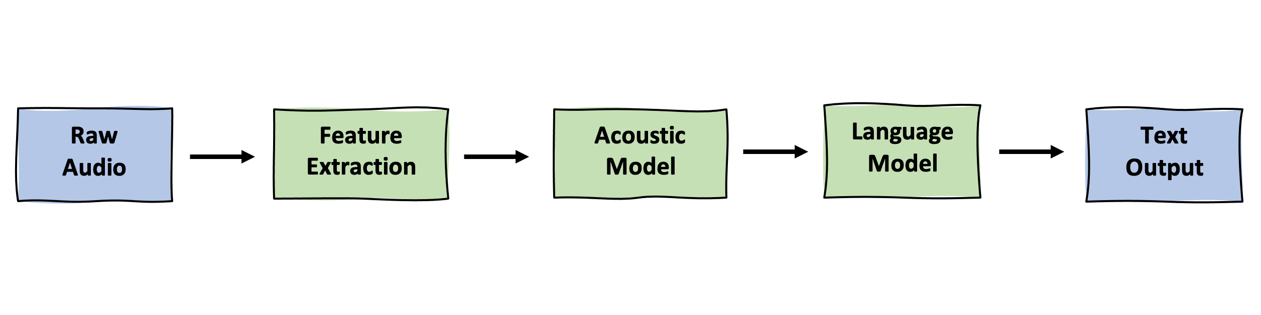
Feature Extraction
Before speech or raw audio is given to models, it needs to be converted into appropriate forms that the models can understand through feature extraction. These representations consists of spectrograms or MFCCs.
Acoustic Model
After features are extracted, these vectors are passed to acoustic models. An acoustic model attempts to map the audio signal to the basic units of speech such as phonemes or graphemes. Implementations of these models include HMMs and neural networks. These linguistic units are elaborated on in the subsequent section.
Language Model
Let’s assume the acoustic model correctly maps the audio to words. Some words may sound the same (homophones: sea vs see) or sound very similar (sheet vs. sea), but have completely different meanings. Language models allow the algorithm to learn the context or meaning of a sentence or a word. One popular and record breaking language model is called BERT.
This article will comprise of the first step in the pipeline which is the decomposition of the components of raw audio into feature representations that can be learned by acoustic models.
Difficulties in ASR
Automatic Speech Recognition is difficult due to a variety of factors in the raw audio itself, uniqueness in individual elocution, ambiguous word boundaries, and lack of context. Let’s take a look these challenges.
Noise
Noise refers to random fluctuations that obscure or do not contain meaningful data or other information. The recognizer should be able to isolate areas of audio signals from the areas of useless noise.
- These include background conversations, microphone static, airplanes flying by, dogs barking, and so forth.
Elocution
Elocution refers to the way an individual pronounces and articulates words. Different people have different elocutions such as variability in pitch, variability in volume, and variability in word speed, and thus it is difficult to account for these many differences.
- For instance, visually and auditorily we can see and hear that ‘speed‘ and ‘speeeeecchhh‘ are spoken in different speeds. It is likely that the pitch and volume are also different. These discrepancies need to be aligned and matched.
Ambiguous Word Boundaries
Unlike written language, speech does not have clear and defined word boundaries. Written text has spaces, commas, and other forms of separation between words. In speech, words seem to overlap each other one after the other.
- "where are the word boundaries ?" vs. "wherearethewordboundaries"
Lack of Context
Generally, conversations flow because people are able to fill in the blanks due to our intrinsic contextual recognizer. Without context, it is difficult to differentiate between two completely different sentences that may sound alike.
- "Can you recognize speech ?" vs. "Can you wreck a nice beach ?"
Physical Properties of Speech
Although there are difficulties in speech recognition, there are physical properties of speech that assist in speech recognition. For instance, we can break speech down into basic units such as graphemes and phonemes.
Phonemes
Phonemes are distinct sounds in language, denoted within slashes i.e. /ah/. In other words, they are the smallest unit of sound. There are about 40 phonemes for American English and 44 phonemes for UK English. For instance, we can break down ‘SPEECH’ into ‘S P IY CH’.
Graphemes
Graphemes are distinct characters in language, denoated within angle brackets i.e. . They are the smallest unit of a writing system. In English, there 250 graphemes, but the smallest grapheme is the set of alphabetical letters (A-Z) plus a space character.
Why can’t we just map Phonemes → Graphemes or vice versa?
There does not exist a 1-to-1 mapping between Phonemes → Graphemes or Graphemes → Phonemes. Multiple phonemes map to the same grapheme and multiple graphemes map to the same phoneme.
The letter c maps to different sounds depending on the word.
- i.e. → /K/ for cat, → /CH/ for chat, and → /S/ for ceremony.
Alternatively, the ‘IY’ sound such as in the word ‘SPEECH’, can be formed with different spellings.
- i.e. /IY/ → for receive, /IY/ → believe, and /IY/ → for speech.
How are these useful?
Although phonemes cannot directly map to graphemes, they are a useful intermediate step for speech processing. This step is called lexical decoding. If we can successfully decode the output of an acoustic model into phonemes, then we can map these phonemes to their words using a lexicon (dictionary mapping) in post-processing steps to form words and sentences.
Additionally, this post-processing step allows us to reduce complexity by mapping to a constant set of values. For high dimensionality problems, problems with a large vocabulary, phonemes can be useful to drastically reduce the number of comparisons between words. However, if the problem has a small vocabulary size, one may opt to use the acoustic model to map directly to words and skip this intermediate step.
If you’d like to incorporate phonemes into your post-postprocessing step, take a look at ARPHABET. It is a well-known phoneme set that was created for speech research.
Signal Analysis
Speech consists of sound waves which are sinusoidal vibrations that travel through the air. Audio input devices such as microphones capture the acoustic energy from these sound waves and record them as audio signals. More on sound.

Here are some basic definitions of wave properties:
Amplitude
- how much acoustic energy is in the sound wave, how loud it is.
- louder sounds have higher amplitudes, while quieter sounds have smaller amplitudes
Frequency
- how many times the wave is repeating itself, measured in Hertz (Hz) or cycles per second
- high-frequency sounds such as sirens has shorter wavelengths, while low frequency sounds such as a low bass have longer wavelengths
Now, let’s take a look at a recorded audio wave.
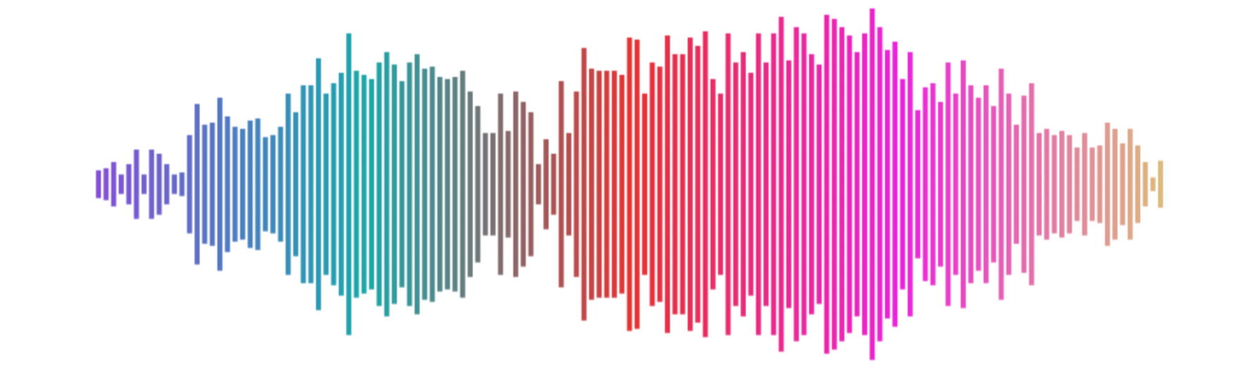
Notice that the shape of this wave doesn’t look a cosine or sine function, shown previously. This is due to the complexity in sound. Sound waves are made of multiple overlapping waves that increase in amplitude when superimposed (added together) through constructive interference and decrease in amplitude (cancel out) through destructive inference.

By looking at only 2 waves, we can already see a more complex and noisier wave start to form when wave 1 and wave 2 are superimposed. In essence, sound waves are made up of many overlapping sound waves and thus can be decomposed into individual, smaller wave components. In other words, resultant_wave = wave1 + wave2 for 2 waves.
Fourier Analysis
Fourier Analysis is the study decomposing mathematical functions into sums of simpler trigonometric functions. Since sound is comprised of oscillating vibrations, we can use Fourier analysis, and Fourier transforms to decompose an audio signal into component sinusoidal functions at varying frequencies.
Fourier transform
A Fourier transform is a mathematical transform that decomposes a time-based pattern into its components.
Here’s a plain-English metaphor:
What does the Fourier Transform do? Given a smoothie, it finds the recipe.
How? Run the smoothie through filters to extract each ingredient.
Why? Recipes are easier to analyze, compare, and modify than the smoothie itself.
How do we get the smoothie back? Blend the ingredients. – source
Using a Fourier transform, we can break complex sound waves into simpler components and process the individual components into useful features before attempting to transcribe the audio into text or perform other objectives.
Fourier transforms are useful tools to extract features from speech into meaningful forms that our models can use. We can use the Fast Fourier Transform (FFT) algorithm to generate a frequency representation of the sound wave by splitting the sound wave into a spectrogram. The spectrogram can then be given to a model to directly predict on or we can further extract features from it before the prediction phase.
Spectrograms
A spectrogram is the frequency domain representation of a wave through time. We’ll take a look at what that means below.
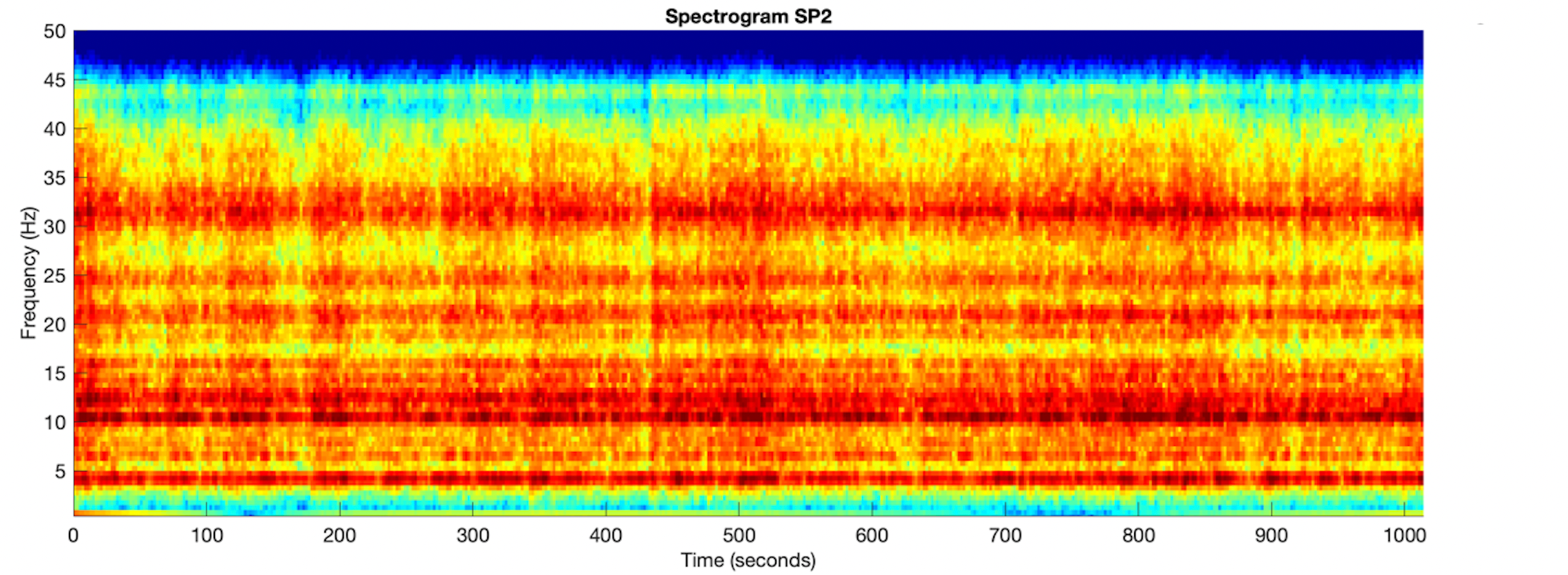
The vertical axis represents the frequency or how fast the wave is moving at time t, defined in the horizontal axis. The color indicates the amplitude of the signal. We are able to line up the spectrogram output with the original audio signal with respect to time.
- Here is a resource that that explains how sounds in spectrograms can be interpreted.
Using an algorithm called the Fast Fourier transform (FFT) algorithm, we can take audio in the form of waves, decompose them into smaller components and visualize the components at each interval of time t in the spectrogram.
- Divide the signal into timeframes
- Split each frame into frequency components with an FFT
- each time frame is now represented as a vector of amplitudes at each frequency
SciPy allows you to easily implement an FFT using the following import statement:
from spicy.fftpack import fftIssues
Although the spectogram gives a complete representation of the sound data, it still contains noise and other variability (mentioned above) that may cloud the data and be more than we actually need. It is crucial to identify and isolate the parts of an audio signal that will actually have predictive power.
Mel Frequency Cepstral Coefficients
The spectogram allowed us to map raw audio into a representation of frequecies. However, we need a way to further filter the noisey audio signal. Notice that audible speech is constrained by both our mouths (that produce sounds) and our ears (that capture sound).
Here’s where Mel Frequency Cepstral Coefficients (MFCCs) come in. Mel Frequency Cepstral Coefficients are extracted from Mel Frequency Analysis and Cepstral Analysis.
Mel Frequency Analysis
To begin, let’s define a relative scale for pitches.
Mel scale
The mel scale (after the word melody)[1] is a perceptual scale of pitches judged by listeners to be equal in distance from one another.
The Mel Scale was developed from studies of pitch perception and allows us to have a measure between pitches. It tells us what pitches people can truly discern.
- For example, pitches 100 Hz and 200 Hz may be perceived to sound farther apart than pitches 1000 Hz and 1100 Hz even though these pairs of pitches both differ by 100 Hz. This result may be because people can distinguish pitches at lower frequencies better.
Dimensionality reduction
Since cannot discern every frequency, sound can be filtered by only keeping the frequencies that can actually be heard. Filtering frequencies out of the range of human listeners can remove irrelevant information, while preserving predictive signals.
Furthermore, if we cannot distinguish between two different frequencies, then these frequencies can be labeled as the same frequency. Notice that spectrograms are on a continuous scale. By converting to a discrete scale by binning frequencies, the total number of frequencies will be reduced.
Mel frequency analysis allows an overall reduction of data dimensionality by filtering noise and discretizing frequencies.
Cepstral Analysis
Human voices vary from person to person even if our anatomy is the same. The production of sound by humans ismade from a combination of "source" and "filter". We’ll see what that means below.
Source-Filter model
The Source-Filter model distinguishes speaker independent and speaker dependent sources of speech.
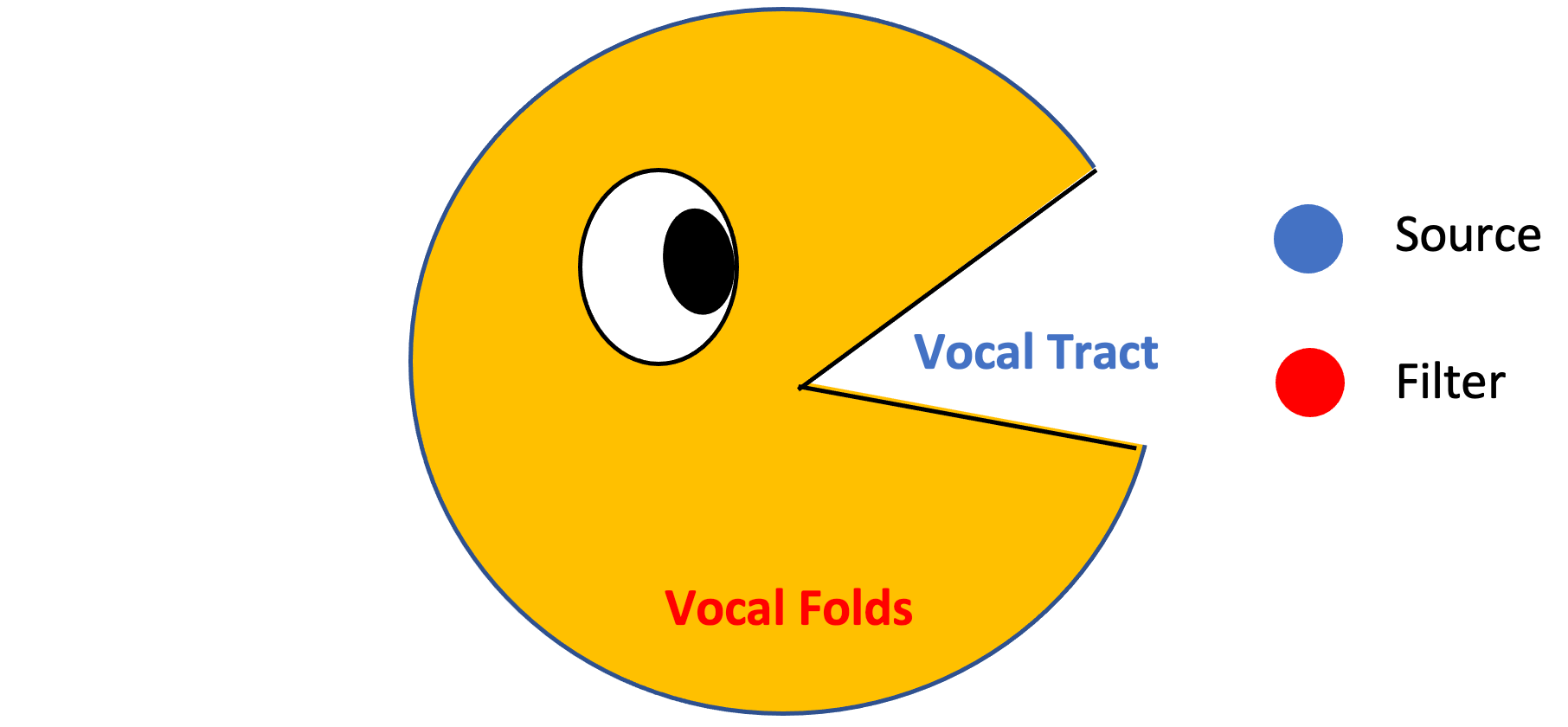
The source, shown in red, represents sound generating parts that are unique to each individual person such as vocal cords or vocal folds. The filter, shown in blue, consists of the vocal tract, that affect the articulation of words used by all people when speaking such as the nasal cavity or the oral cavity. The goal is to focus on the articulation of words (vocal folds) and to ignore the parts (the vocal tract) that are independent of speak.
Cepstral analysis allows us to seperate the source and filter. Mainly it allows us to drop the source and perserve the shape of the sound made by the filter. The source and the filter motivate the idea behind Cepstral analysis. Essentially, the source is multiplied by the filter to form the signal, which can be then transfers into the frequency domain through an FFT and so forth.
If you would like to see the theory, take a look at the following:
Cepstral Analysis of Speech Theory
Combining Features
Mel Frequency Analysis and Cepstral Analysis results in about 12 MCFF features. Additionally, MFCC deltas (changes in frequencies) or MFCC delta-deltas (changes in changes in frequencies) may be useful features for automatic speech recognition. These additional features can double or triple the total number of MFCC features. They have also been shown to give better results in ASR.
Tutorial on MFCC implementation and MFCC deltas
The main takeaway is that MCFF features result in a greatly reduced number of frequencies. MCFFs filter noise unlike a spectrogram and hone in on the parts of the signal that have greater predictive power.
Conclusion
In conclusion, Automatic Speech Recognition comes with many challenges, but by understanding the basic components of speech, we can simplify the problem. Raw audio waves can be converted into feature representations, then further reduced using knowledge of sound waves and domain knowledge of physical human constraints of sound. These techniques result in a cleaner and stronger signal that can help us more efficiently train our acoustic models.


