
Decision trees represent a connecting series of tests that branch off further and further down until a specific path matches a class or label. They’re kind of like a flowing chart of coin flips, if/else statements, or conditions that when met lead to an end result. Decision trees are incredibly useful for classification problems in machine learning because it allows data scientists to choose specific parameters to define their classifiers. So whether you’re presented with a price cutoff or target KPI value for your data, you have the ability to sort data at multiple levels and create accurate prediction models.
Now there are many, many applications that utilize decision trees but for this article, I’m going to focus on using decision trees to make business decisions. This one involves gauging customer interest in new products and we’ll be using data from an online coffee beans distributor!
Problem:

Your client, RR Diner Coffee, is a US-based retailer that sells specialty coffee beans all over the world. They’re looking to add a new product from a highly selective brand. This new addition will seriously boost sales and improve their reputation, but they need to ensure that the product will actually sell. In order to add this product, you will need to prove to your client that at least 70% of your customers are likely to purchase it. Luckily for you, your marketing team sent out a survey and you’ve got a decent amount of data to work with. Let’s take a look.
Exploring the Data

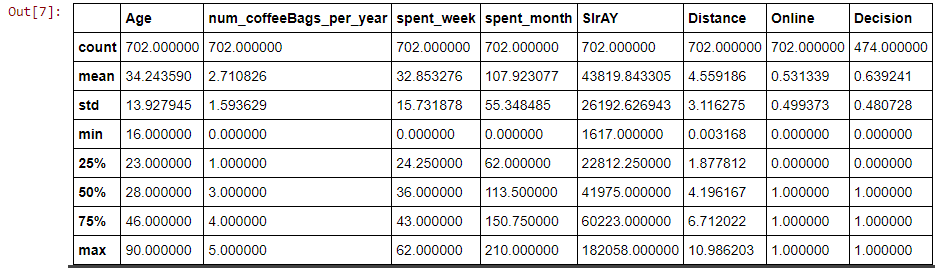
We will definitely need to clean up our data before moving on but just by looking at the data, we can get an idea of what to do with it. What’s very handy about this data is that because of the ‘Decision’ column we already know whether or not some customers will purchase this new product – because we don’t have to make any guesses for our training data we can make a supervised model. Any of these other features could be useful when determining what kind of customer says ‘YES’ but we’ll figure that out later.
To clean this data all I did was:
- Change some of the column names to make it easier to understand
- Make sure all the gender responses are in the same format, like turning ‘Male’, ‘m’, ‘M’, and ‘MALE’ all into ‘Male’ and vice versa.
- Change the 1.0s and 0.0s in the Decision column to ‘YES’ and ‘NO’ respectively, leaving the null data for now.
Now that we know what our data looks like and what approach we can take let’s move on to making train/test splits for our model
Train/Test Splits
Since there are only 702 entries, I wanted to save as much data as possible, even the ones with a null Decision. For this train/test split though, I created a subset of data where the Decision value was not null and called it NOPrediction.
And just like that, we’ve got train/test splits that we can use to evaluate our models. Now let’s move on to the real show: decision tree models!
Models
Just like with every machine learning method there are tons of varieties to choose from when selecting a model. I’m just going to show you some of the ones I tried out in this project but you should read more to find out which ones will work best for you! Scikit-learn’s site has a ton of great documentation: check it out here.
Entropy Model
You might remember from high school physics that entropy measures disorder or randomness in a system. When working with decision trees, you’re going to deal with a lot of randomnesses but it’s your job, as a data scientist, to make prediction models with minimal entropy. The basic entropy model seeks to start from the top of the tree with maximum entropy and work its way down to the roots where you’ll have minimal entropy – this is how you can accurately categorize your data. This is much easier explained visually so let me show you what I mean.
The output should look something like this:

If you start from the top, you can see that as your work your way down the model is making True and False decisions. As these decisions branch off, entropy is getting lower and we’re able to create clearly defined clusters of data.
In this instance, we never defined a max depth or gave the model any other parameters, so this version is the most accurate with a balanced accuracy score of 98.7%. Sometimes, though, it’s good to sacrifice some accuracy for the sake of time and computer processing limits. Like in this example, where we set the maximum depth to 3:

This model has fewer decisions to make and produces a balanced accuracy score of 86.5%. That’s still a really solid prediction model with just half of the decisions from the model with no maximum depth. You can probably see what I’m saying now. If you’re looking for the most accurate model where time and computing power aren’t an issue: there’s no need to set a maximum depth. But, if you’re in a time crunch or have limited resources: setting a maximum depth will save you a lot of time and award you with very similar results!
Gini Impurity Model
Just like the entropy model, this decision tree model seeks to minimize any randomness when categorizing data. However, unlike the previous two models, the Gini Impurity model doesn’t use logarithmic functions and can save you a lot of computing power over time. Here’s the difference between the two:

The setup is very similar to the entropy model, let’s see how it performs.
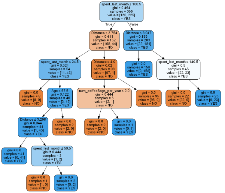
With this, we’ve got a balanced accuracy of 98.1% which is just slightly less accurate than the first entropy model. Just like with the entropy model, you can also set a maximum depth for Gini decision trees.

This model surprisingly has a balanced accuracy of 96.9%! Only a 1.2% difference from the original Gini model with far fewer decisions.
Each model has its own sets of pros and cons and there are others to explore besides these four examples. Which one would you pick? In my opinion, the Gini model with a maximum depth of 3 gives us the best balance of good performance and highly accurate results. There are definitely situations where the highest accuracy or the fewest total decisions is preferred. As a data scientist, it’s up to you to choose which is more important for your project!
Making a Prediction
Now that we’ve got our models created, let’s use them! To prove that RR Diner’s coffee will have interest from at least 70% of our customers we’ll have to feed some new data into our prediction model. Remember how in our dataset we only had 474/702 people actually make a decision? What if we use the other 228 entries for our prediction? We’ll have to set up a new dataframe, add some dummy variables, then feed them into the model. Here’s what that looks like:
This outputs an array of 45NO and 183 YES. If we use value_counts() the ‘Decision’ column of our original dataset we get 151 NO and 323 YES. Now we can just add it all together:
- 183 YES + 323 YES = 506 YES
- 506 YES / 702 TOTAL CUSTOMERS = 0.72
That means that according to the survey we ran and predictions from our model, 72% of our customers would be interested in purchasing RR Diner coffee! In this case, we’ve met the criteria set by the supplier and should be able to add their product to our business. You can even add that our prediction model is over 96% accurate if you really want to impress them. Who knows, securing a deal like this could possibly get you a bonus or even a promotion; Data Science is an incredibly valuable asset in the business world.
Conclusion
I hope that from this example you’ve learned a good amount about decision trees and how you can use them to help make accurate predictions for you or your business! There are many, many other interesting things about decision trees that I didn’t mention, like random forest models or using precision/recall scores when measuring overall accuracy. I’d love to write more about them in the future, but for now, there are plenty of great resources out there to learn even more about predictive analysis. Check out scikit-learn’s documentation for a real deep dive, or this informative video from Edureka! if you want to learn even more!
As always, thank you so much for reading this article! If you like my content please consider following me here on medium as I’m looking to post even more data science content in the future. Hope you have a great day! 
Follow me!-https://bench-5.medium.com/


