A Loss Function Suitable for Class Imbalanced Data: "Focal Loss"

Foggy Afternoon in Nagano, Japan (Image: Author's Own Work) — Foggy Afternoon in Nagano, Japan (Image: Author’s Own Work)

Class Imbalance:

In machine learning sometimes we are dealt with a very good hand like MNIST fashion data or CIFAR-10 data where the examples of each class in the data-set are well balanced. What happens if in a Classification problem the distribution of examples across the known classes are biased or skewed ? Such problems with severe to slight bias in the data-set are common and today we will discuss an approach to handle such class imbalanced data. Let’s consider an extreme case of imbalanced data-set of mails and we build a classifier to detect spam mails. Since spam mails are relatively rarer, let’s consider 5% of all mails are spams. If we just a write a simple one line code as –

def detectspam(mail-data):

 return 'not spam'

This will give us right answer 95% of time and even though this is an extreme hyperbole but you get the problem. Most importantly, training any model with this data will lead to high confidence prediction of the general mails and due to extreme low number of spam mails in the training data, the model will likely not learn to predict the spam mails correctly. This is why precision, recall, F1 score, ROC/AUC curves are the important metrics that truly tell us the story. As you have already guessed one way to reduce this issue is to do sampling to balance the data-set so that classes are balanced. There are several other ways to address class imbalance problem in machine learning and an excellent comprehensive review has been put together by Jason Brownlee, check it here.

Class Imbalance in Computer Vision:

In case of computer vision problem, this class imbalance problem can be more critical and here we discuss how the authors approached object detection tasks that lead to the development of Focal Loss. In case of Fast R-CNN type of algorithms, first we run an image through ConvNet to obtain a feature map and then region proposal is performed (generally around 2K regions) on the high resolution feature map. These are 2-stage detectors and when the Focal Loss paper was introduced the intriguing question was whether one stage detector like YOLO or SSD could obtain same accuracy as 2-stage detectors? One stage detectors were fast but the accuracy during that time was around 10–40% of the 2-stage detectors. The authors suggested that class imbalance during training as the main obstacle that prevents the one stage detectors to obtain same accuracy as 2-stage detectors.

Figure 1: Class Imbalance in Object Detection (Source: Ref. [2])

An example of such class imbalance is shown in the self-explanatory Figure 1, which is taken from the presentation itself by the original authors. They found that one stage detectors perform better when there are higher number of bounding boxes covering the space of possible objects. But this approach caused a major problem as the foreground and background data are not equally distributed. For example if we consider 20000 bounding boxes mostly 7–10 of them will actually contain any info about the object and the remaining will be containing background and, mostly they will be easy to classify but uninformative. Here, the authors found out that Loss function (e.g. Cross-Entropy) is the main reason that the easy examples will distract the training. Below is a pictorial representation

Fig. 2: Class Imbalance and Cross-Entropy Loss (Image by Author).

Even though the wrongly classified samples are penalized more (red arrow in fig. 1) than the correct ones (green arrow), in the dense object detection settings, due to the imbalanced sample size, the loss function is overwhelmed with background (easy samples). The Focal Loss addresses this problem and it is designed in such a way so that it reduces the loss (‘down-weight’) for the easy examples and thus the network can focus on training the hard examples. Below is the definition of Focal Loss –

In focal loss, there’s a modulating factor multiplied to the Cross-Entropy loss. When a sample is misclassified, p (which represents model’s estimated probability for the class with label y = 1) is low and the modulating factor is near 1 and, the loss is unaffected. As p→1, the modulating factor approaches 0 and the loss for well-classified examples is down-weighted. The effect of γ parameter is shown in the plot below –

Fig. 3: Focal Loss Compared with Cross Entropy Loss (Image by Author). Codes are available in my Notebook [Ref. 3]

To quote from the paper –

The modulating factor reduces the loss contribution from easy examples and extends the range in which an example receives low loss.

To understand this we will compare Cross-Entropy (CE) loss and Focal Loss using the definition above with γ = 2. Consider true value 1.0, and we consider 3 prediction values 0.90 (close), 0.95 (very close), 0.20 (far from true). Let’s see the loss values below using TensorFlow—

CE loss when pred is close to true:  0.10536041
CE loss when pred is very close to true:  0.051293183
CE loss when pred is far from true:  1.6094373

focal loss when pred is close to true:  0.0010536041110754007
focal loss when pred is very close to true:  0.00012823295779526255
focal loss when pred is far from true:  1.0300399017333985

Here we see that compared to CE loss, the modulating factor in focal loss plays an important role. When prediction is close to the truth the loss is penalized way more than when when it is far. Importantly when prediction is 0.90 focal loss will be 0.01 × CE loss but when prediction is 0.95, focal loss will be around 0.002 × CE loss. Now we get a picture how focal loss reduces the loss contribution from easy examples and extends the range in which an example receives low loss. This can also be seen from fig. 3. Now we will use a real-world class imbalanced data-set and see focal loss in action.

Credit-Card Fraud: Class Imbalance Data-Set:

Data-set Description: Here I have considered an extreme class-imbalanced data-set available in Kaggle and the data-set contains transactions made by credit cards in September 2013 by European cardholders. Let’s use pandas –

This data-set presents transactions that occurred in two days and we have 284,807 number of transactions. Features V1, V2,…V28 are the principal components obtained with PCA (original features are not provided due to confidential issues) and the only features which have not been transformed with PCA are ‘Time’ and ‘Amount’. Feature ‘Time’ contains the seconds elapsed between each transaction and the first transaction in the dataset and the feature ‘Amount’ is the transaction amount. Feature ‘Class’ is the response variable and it takes value 1 in case of fraud and 0 otherwise.

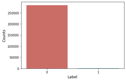
Fig. 4: Distribution of Real(0) and Fraud(1) transactions in the data-set. Image by Author.

Class Imbalance: Let’s plot the distribution of the ‘Class’ feature which tells us how many transactions are real and fake. As shown in figure 4 above, overwhelming numbers of transactions are real. Let’s get the numbers with this simple piece of code –

print ('real cases:', len(credit_df[credit_df['Class']==0]))

print ('fraud cases: ', len(credit_df[credit_df['Class']==1]))


>>> real cases:  284315
    fraud cases:  492

So the class imbalance ratio is about 1:578, so for 578 real transactions we have one fraud case. First let’s use a simple neural network with cross-entropy loss to predict fraud and real transactions. But before that a little examination tells us that ‘Amount’ and ‘Time’ features are not scaled whereas other features ‘V1’, ‘V2’…etc are scaled. Here we can use StandardScaler/RobustScaler to scale these features and since RobustScaler are robust to outliers, I chose this standardization technique.

Let’s now choose the features and label as below –

X_labels = credit_df.drop(['Class'], axis=1)
y_labels = credit_df['Class']

X_labels = X_labels.to_numpy(dtype=np.float64)

y_labels = y_labels.to_numpy(dtype=np.float64)


y_lab_cat = tf.keras.utils.to_categorical(y_labels, num_classes=2, dtype='float32')

For the train-test split we use stratify to keep the ratio of labels –

x_train, x_test, y_train, y_test = train_test_split(X_labels, y_lab_cat, test_size=0.3, stratify=y_lab_cat, shuffle=True)

Now we build a simple neural-net model with 3 dense layers –

def simple_model():

   input_data = Input(shape=(x_train.shape[1], ))

   x = Dense(64)(input_data)

   x = Activation(activations.relu)(x)

   x = Dense(32)(x)

   x = Activation(activations.relu)(x)

   x = Dense(2)(x)

   x = Activation(activations.softmax)(x)

   model = Model(inputs=input_data, outputs=x, name='Simple_Model')

   return model

Compile the model with categorical cross-entropy as loss—

simple_model.compile(optimizer=Adam(learning_rate=5e-3), loss='categorical_crossentropy', metrics=['acc'])

Train the model –

simple_model.fit(x_train, y_train, validation_split=0.2, epochs=5, shuffle=True, batch_size=256)

To truly understand the performance of the model, we need to plot the confusion matrix along with the precision, recall and F1 scores –

Fig. 5: Confusion Matrix, Precision, Recall, F1 Scores with Cross Entropy Loss (Image by Author)

We see from the confusion matrix and other performance metric scores that as expected the network does extremely good to classify the real transactions but the recall value is below 50% for the fraud class. Our target is to test without changing anything except the loss function can we get better values for the performance metrics ?

Using Focal Loss:

First let’s define the focal loss with alpha and gamma as hyper-parameters and to do this I have used the tfa module which is a functionality for TensorFlow maintained by SIG-addons (tfa). Under this module among the additional losses, there’s an implementation of Focal Loss and first we import as below –

import tensorflow_addons as tfa

fl = tfa.losses.SigmoidFocalCrossEntropy(alpha, gamma)

Using this, let’s define a custom loss function that can be used as a proxy for ‘Focal Loss’ for this specific problem with two classes—

def focal_loss_custom(alpha, gamma):

   def binary_focal_loss(y_true, y_pred):

      fl = tfa.losses.SigmoidFocalCrossEntropy(alpha=alpha, gamma=gamma)

      y_true_K = K.ones_like(y_true)

      focal_loss = fl(y_true, y_pred)

      return focal_loss

   return binary_focal_loss

We now just repeat the steps above for model definition, compile and fit but this time using focal loss as below –

simple_model.compile(optimizer=Adam(learning_rate=5e-3),       loss=focal_loss_custom(alpha=0.2, gamma=2.0), metrics=['acc'])

For alpha and gamma parameters, I have just used the values suggested in the paper (however the problem is different) and different values need to be tested.

simple_model.fit(x_train, y_train, validation_split=0.2, epochs=5, shuffle=True, batch_size=256)

Using Focal Loss we see an improvement as below –

Fig. 6: Confusion Matrix, Precision, Recall, F1 Scores with Focal Loss (Image by Author)

We see using ‘Focal Loss’ the performance metrics improved considerably and we could detect more ‘Fraud’ transactions (101/148) correctly compared to the previous case (69/148).

Here in this post we discuss Focal Loss and how it can improve classification task when the data is highly imbalanced. To demonstrate Focal Loss in action we used Credit Card Transaction data-set which is highly biased towards real transactions and showed how Focal Loss improves the classification performance.

I would also like to mention that , in my research with gamma-ray data we are trying to classify Active Galactic Nuclei (AGN) from Pulsars (PSR) and the gamma-ray sky is mostly populated by AGNs. The picture below is an example of such a simulated sky. This is also an example of class-imbalanced data-set in computer vision.