CAUSAL DATA SCIENCE
AB tests or randomized controlled trials are the gold standard in Causal Inference. By randomly exposing units to a treatment we make sure that treated and untreated individuals are comparable, on average, and any outcome difference we observe can be attributed to the treatment effect alone.
However, often the treatment and control groups are not perfectly comparable. This could be due to the fact that randomization was not perfect or available. It is not always possible to randomize a treatment, for ethical or practical reasons. Even when we can, sometimes we do not have enough individuals or units, so that differences between groups are seizable. This happens often, for example, when randomization is not done at the individual level, but at a higher level of aggregation like zip codes, counties, or even states.
In these settings, we can still recover a causal estimate of the treatment effect if we have enough information about individuals, by making the treatment and control group comparable, ex-post. In this blog post, we are going to introduce and compare different procedures to estimate causal effects in presence of imbalances between treatment and control groups that are fully observable. In particular, we are going to analyze weighting, matching, and regression procedures.
Example
Assume we had a blog on Statistics and causal inference. To improve user experience, we are considering releasing a dark mode, and we would like to understand whether this new feature increases the time users spend on our blog.

We are not a sophisticated company, therefore we do not run an A/B test but we simply release the dark mode and we observe whether users select it or not and the time they spend on the blog. We know that there might be selection: users that prefer the dark mode could have different reading preferences and this might complicate our causal analysis.
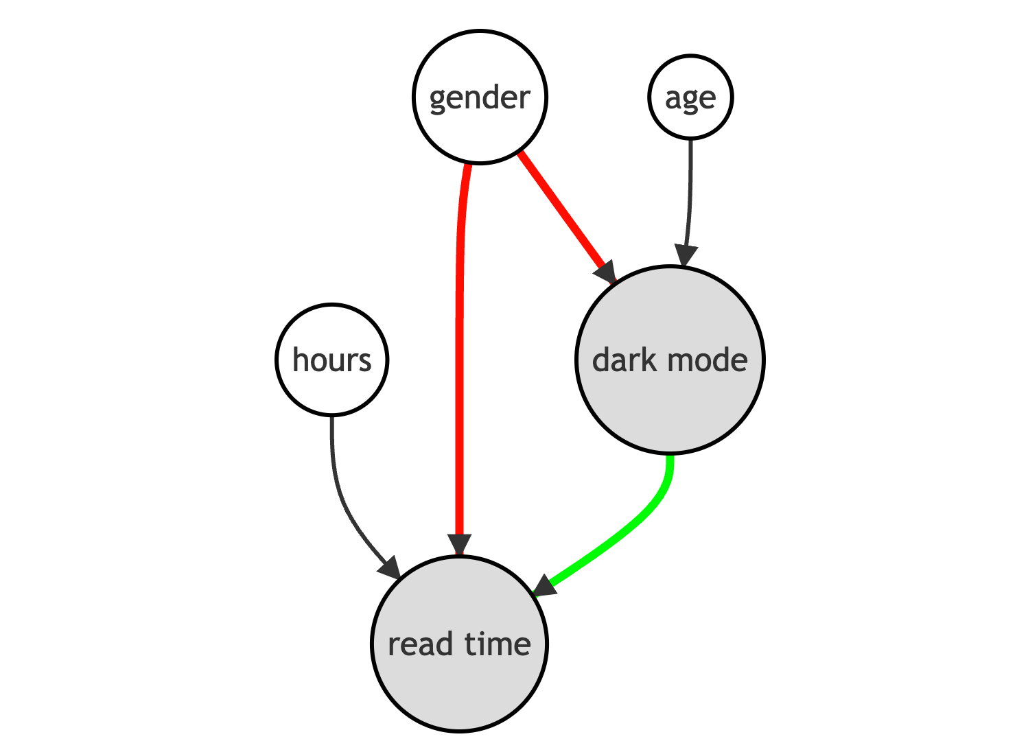
We can represent the data generating process with the following Directed Acyclic Graph (DAG).
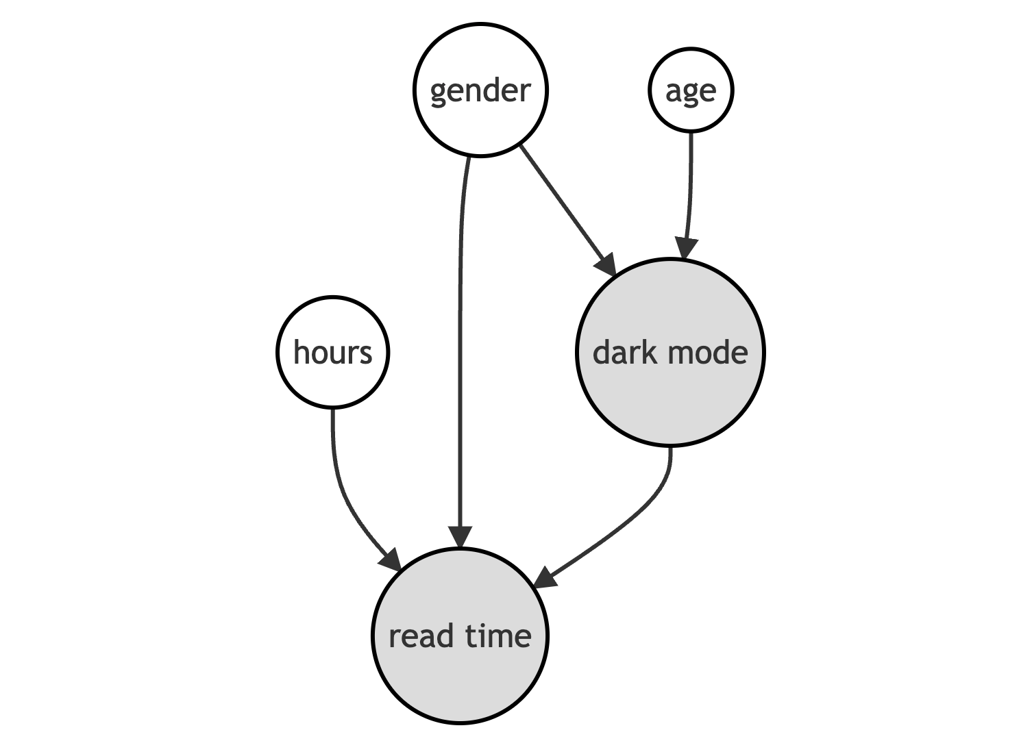
We generate the simulated data using the data generating process dgp_darkmode() from [src.dgp](https://github.com/matteocourthoud/Blog-Posts/blob/main/notebooks/src/dgp.py). I also import some plotting functions and libraries from [src.utils](https://github.com/matteocourthoud/Blog-Posts/blob/main/notebooks/src/utils.py).
from src.utils import *
from src.dgp import dgp_darkmode
df = dgp_darkmode().generate_data()
df.head()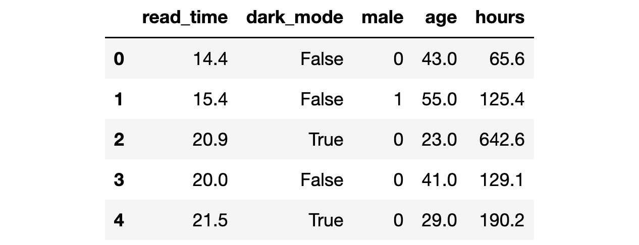
We have information on 300 users for whom we observe whether they select the dark_mode (the treatment), their weekly read_time (the outcome of interest) and some characteristics like gender, age and total hours previously spend on the blog.
We would like to estimate the effect of the new dark_mode on users’ read_time. If we were running an A/B test or randomized control trial, we could just compare users with and without the dark mode and we could attribute the difference in average reading time to the dark_mode. Let’s check what number we would get.
np.mean(df.loc[df.dark_mode==True, 'read_time']) - np.mean(df.loc[df.dark_mode==False, 'read_time'])-0.4446330948042103Individuals that select the dark_mode spend on average 0.44 hours less on the blog, per week. Should we conclude that dark_mode is a bad idea? Is this a causal effect?
We did not randomize the dark_mode so that users that selected it might not be directly comparable with users that didn’t. Can we verify this concern? Partially. We can only check characteristics that we observe, gender, age and total hours in our setting. We cannot check if users differ along other dimensions that we don’t observe.
Let’s use the create_table_one function from Uber’s [causalml](https://causalml.readthedocs.io/) package to produce a covariate balance table, containing the average value of our observable characteristics, across treatment and control groups. As the name suggests, this should always be the first table you present in causal inference analysis.
from causalml.match import create_table_one

X = ['male', 'age', 'hours']
table1 = create_table_one(df, 'dark_mode', X)
table1
There seems to be some difference between the treatment (dark_mode) and control group. In particular, users that select the dark_mode are younger, have spent fewer hours on the blog and they are more likely to be males.
Another way to visually observe all the differences at once is with a paired violinplot. The advantage of the paired violinplot is that it allows us to observe the full distribution of the variable (approximated via kernel density estimation).
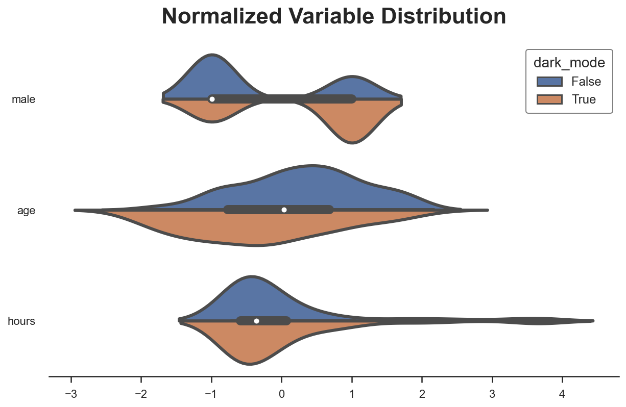
The insight of the violinplot is very similar: it seems that users that select the dark_mode are different from users that don’t.
Why do we care?
If we do not control for the observable characteristics, we are unable to estimate the true treatment effect. In short, we cannot be certain that the difference in the outcome, read_time, can be attributed to the treatment, dark_mode, instead of other characteristics. For example, it could be that males read less and also prefer the dark_mode, therefore we observe a negative correlation even though dark_mode has no effect on read_time (or even positive).
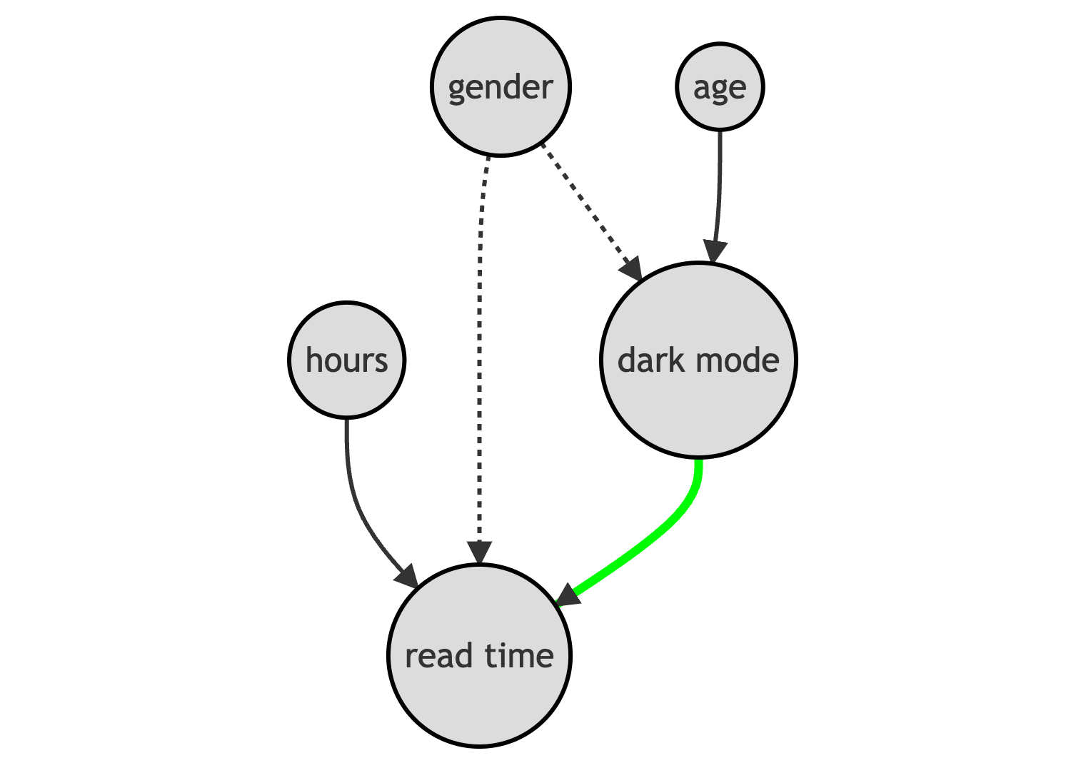
In terms of Directed Acyclic Graphs, this means that we have a backdoor path that we need to block in order for our analysis to be causal.
How do we block backdoor paths? By conditioning the analysis on those intermediate variables, in our case gender. The conditional analysis allows us to recover the causal effect of the dark_mode on read_time. Further conditioning the analysis on age and hours allows us to increase the precision of our estimates but does not impact the causal interpretation of the results.
How do we condition the analysis on gender, age and hours? We have some options:
- Matching
- Propensity score weighting
- Regression with control variables
Let’s explore and compare them!
Conditional Analysis
We assume that for a set of subjects i = 1, …, n we observed a tuple (Dᵢ, Yᵢ, Xᵢ) comprised of
- a treatment assignment Dᵢ ∈ {0,1} (
dark_mode) - a response Yᵢ ∈ ℝ(
read_time) - a feature vector Xᵢ ∈ ℝⁿ (
gender,ageandhours)
Assumption 1: unconfoundedness (or ignorability, or selection on observables)

i.e. conditional on observable characteristics X, the treatment assignment D is as good as random. What we are effectively assuming is that there are no other characteristics that we do not observe that could impact both whether a user selects the dark_mode and their read_time. This is a strong assumption that is more likely to be satisfied the more individual characteristics we observe.
Assumption 2: overlap (or common support)

i.e. no observation is deterministically assigned to the treatment or control group. This is a more technical assumption that basically means that for any level of gender, age or hours, there could exist an individual that selects the dark_mode and one that doesn’t. Contrary to the unconfoundedness assumption, the overlap assumption is testable.
Matching
The first and most intuitive method to perform conditional analysis is matching.
The idea of matching is very simple. Since we are not sure whether, for example, male and female users are directly comparable, we do the analysis within gender. Instead of comparing read_time across dark_mode in the whole sample, we do it separately for male and female users.
df_gender = pd.pivot_table(df, values='read_time', index='male', columns='dark_mode', aggfunc=np.mean)
df_gender['diff'] = df_gender[1] - df_gender[0]
df_gender
Now the effect of dark_mode seems reversed: it is negative for male users (-0.03) but positive and larger for female users (+1.93), suggesting a positive aggregate effect, 1.93 – 0.03 = 1.90 (assuming an equal proportion of genders)! This sign reversal is a very classical example of Simpson’s Paradox.
This comparison was easy to perform for gender, since it is a binary variable. With multiple variables, potentially continuous, matching becomes much more difficult. One common strategy is to match users in the treatment group with the most similar user in the control group, using some sort of nearest neighbor algorithm. I won’t go into the algorithm details here, but we can perform the matching with the NearestNeighborMatch function from the causalml package.
The NearestNeighborMatch function generates a new dataset where users in the treatment group have been matched 1:1 (option ratio=1) to users in the control group.
from causalml.match import NearestNeighborMatch

psm = NearestNeighborMatch(replace=True, ratio=1, random_state=1)
df_matched = psm.match(data=df, treatment_col="dark_mode", score_cols=X)
Are the two groups more comparable now? We can produce a new version of the balance table.
table1_matched = create_table_one(df_matched, "dark_mode", X)
table1_matched
Now the average differences between the two groups have shrunk by at least a couple of orders of magnitude. However, note how the sample size has slightly decreased (300 → 208) since (1) we only match treated users and (2) we are not able to find a good match for all of them.
We can visually inspect distributional differences with the paired violinplot.
plot_distributions(df_matched, X, "dark_mode")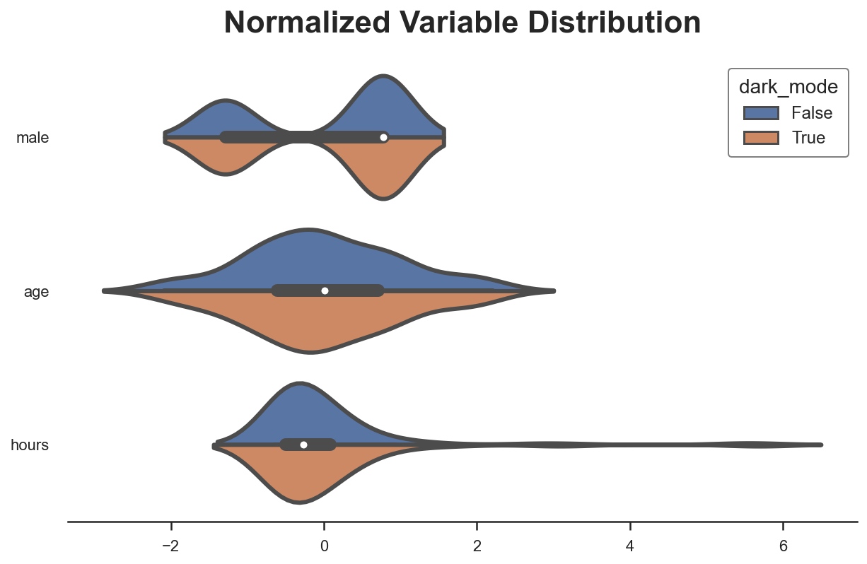
A popular way to visualize pre- and post-matching covariate balance is the balance plot that essentially displays the standardized mean differences before and after matching, for each control variable.

As we can see, now all differences in observable characteristics between the two groups are essentially zero. We could also compare the distributions using other metrics or test statistics, such as the Kolmogorov-Smirnov test statistic.
How do we estimate the treatment effect? We can simply do a difference in means. An equivalent way that automatically provides standard errors is to run a linear regression of the outcome, read_time, on the treatment, dark_mode.
Note that, since we have performed the matching for each treated user, the treatment effect we are estimating is the average treatment effect on the treated (ATT), which can be different from the average treatment effect if the treated sample differs from the overall population (which is likely to be the case, since we are doing matching in the first place).
smf.ols("read_time ~ dark_mode", data=df_matched).fit().summary().tables[1]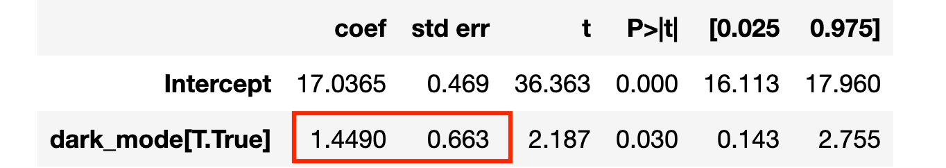
The effect is now positive, and statistically significant at the 5% level.
Note that we might have matched multiple treated users with the same untreated user, violating the independence assumption across observations and, in turn, distorting inference. We have two solutions:
- cluster standard errors at the pre-matching individual level
- compute standard errors via bootstrap (preferred)
We implement the first and cluster standard errors by the original individual identifiers (the dataframe index).
smf.ols("read_time ~ dark_mode", data=df_matched)
    .fit(cov_type='cluster', cov_kwds={'groups': df_matched.index})
    .summary().tables[1]
The effect is less statistically significant now.
Propensity Score
Rosenbaum and Rubin (1983) proved a very powerful result: if the strong ignorability assumption holds, it is sufficient to condition the analysis on the probability of treatment, the propensity score, in order to have conditional independence.

Where e(Xᵢ) is the probability of treatment of individual i, given the observable characteristics Xᵢ.

Note that in an A/B test the propensity score is constant across individuals.
The result from Rosenbaum and Rubin (1983) is incredibly powerful and practical, since the propensity score is a one-dimensional variable, while the control variable X might be very high-dimensional.
Under the unconfoundedness assumption introduced above, we can rewrite the average treatment effect as

Note that this formulation of the average treatment effect does not depend on the potential outcomes Yᵢ⁽¹⁾ and Yᵢ⁽⁰⁾, but only on the observed outcomes Yᵢ.
This formulation of the average treatment effect implies the Inverse Propensity Weighted (IPW) estimator which is an unbiased estimator for the average treatment effect τ.

This estimator is unfeasible since we do not observe the propensity scores e(Xᵢ). However, we can estimate them. Actually, Imbens, Hirano, Ridder (2003) show that you should use the estimated propensity scores even if you knew the true values (for example because you know the sampling procedure). The idea is that, if the estimated propensity scores are different from the true ones, this can be informative in the estimation.
There are several possible ways to estimate a probability, the simplest and most common one being logistic regression.
from sklearn.linear_model import LogisticRegressionCVdf["pscore"] = LogisticRegressionCV().fit(y=df["dark_mode"], X=df[X]).predict_proba(df[X])[:,1]It is best practice, whenever we fit a prediction model, to fit the model on a different sample with respect to the one that we use for inference. This practice is usually called cross-validation or cross-fitting. One of the best (but computationally expensive) cross-validation procedures is leave-one-out (LOO) cross-fitting: when predicting the value of observation i, we use all observations except for i. We implement the LOO cross-fitting procedure using the cross_val_predict and LeaveOneOut functions from the [skearn](https://scikit-learn.org/) package.
from sklearn.model_selection import cross_val_predict, LeaveOneOutdf['pscore'] = cross_val_predict(estimator=LogisticRegressionCV(),
X=df[X],
y=df["dark_mode"],
cv=LeaveOneOut(),
method='predict_proba',
n_jobs=-1)[:,1]An important check to perform after estimating propensity scores is plotting them, across the treatment and control groups. First of all, we can then observe whether the two groups are balanced or not, depending on how close the two distributions are. Moreover, we can also check how likely it is that the overlap assumption is satisfied. Ideally, both distributions should span the same interval.
sns.histplot(data=df, x='pscore', hue='dark_mode', bins=30, stat='density', common_norm=False).
    set(ylabel="", title="Distribution of Propensity Scores");
As expected, the distribution of propensity scores between the treatment and control groups is significantly different, suggesting that the two groups are hardly comparable. However, the two distributions span a similar interval, suggesting that the overlap assumption is likely to be satisfied.
How do we estimate the average treatment effect?
Once we have computed the propensity scores, we just need to weight observations by their respective propensity score. We can then either compute a difference between the weighted read_time averages, or run a weighted regression of read_time on dark_mode using the wls function (weighted least squares).
w = 1 / (df["pscore"] * df["dark_mode"] + (1-df["pscore"]) * (1-df["dark_mode"]))
smf.wls("read_time ~ dark_mode", weights=w, data=df).fit().summary().tables[1]
The effect of dark_mode is now positive and almost statistically significant, at the 5% level.
Note that the wls function automatically normalizes weights so that they sum to 1, which greatly improves the stability of the estimator. In fact, the unnormalized IPW estimator can be very unstable when the propensity scores approach zero or one.
Regression with Control Variables
The last method we are going to review today is linear regression with control variables. This estimator is extremely easy to implement since we just need to add user characteristics – gender, age and hours – to the regression of read_time on dark_mode.
smf.ols("read_time ~ dark_mode + male + age + hours", data=df).fit().summary().tables[1]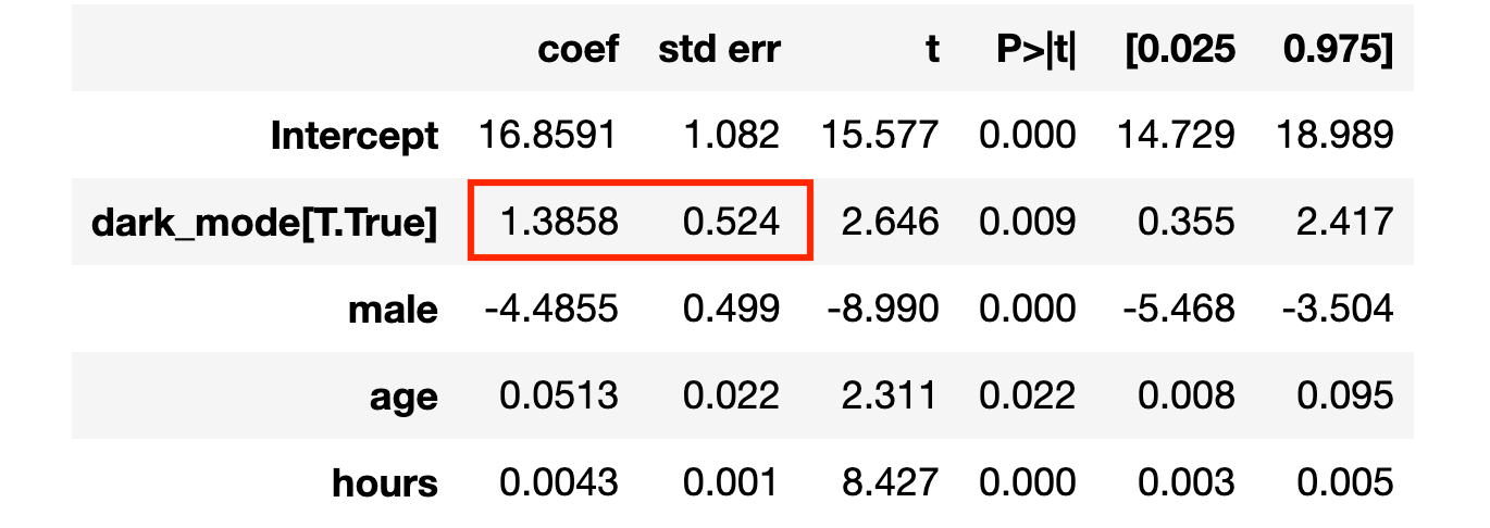
The average treatment effect is again positive and statistically significant at the 1% level!
Comparison
How are the different methods related to each other?
IPW and Regression
There is a tight connection between the IPW estimator and linear regression with covariates. This is particularly evident when we have a one-dimensional, discrete covariate X.
In this case, the estimand of IPW (i.e. the quantity that IPW estimates) is given by

The IPW estimand is a weighted average of the treatment effects τₓ, where the weights are given by the treatment probabilities.
The estimand of linear regression with control variables is

The OLS estimand is a weighted average of the treatment effects τₓ, where the weights are given by the variances of the treatment probabilities. This means that linear regression is a weighted estimator, that gives more weight to observations that have characteristics for which we observe more treatment variability. Since a binary random variable has the highest variance when its expected value is 0.5, OLS gives the most weight to observations that have characteristics for which we observe a 50/50 split between the treatment and control group. On the other hand, if for some characteristics we only observe treated or untreated individuals, those observations are going to receive zero weight. I recommend Chapter 3 of Angrist and Pischke (2009) for more details.
IPW and Matching
As we have seen in the IPW section, the result from Rosenbaum and Rubin (1983) tells us that we do not need to perform the analysis conditional on all the covariates X, but it is sufficient to condition on the propensity score e(X).
We have seen how this result implies a weighted estimator but it also extends to matching: we do not need to match observations on all the covariates X, but it is sufficient to match them on the propensity score e(X). This method is called propensity score matching.
psm = NearestNeighborMatch(replace=False, random_state=1)
df_ipwmatched = psm.match(data=df, treatment_col="dark_mode", score_cols=['pscore'])
As before, after matching, we can simply compute the estimate as a difference in means, remembering that observations are not independent and therefore we need to be cautious when doing inference.
smf.ols("read_time ~ dark_mode", data=df_ipwmatched)
    .fit(cov_type='cluster', cov_kwds={'groups': df_ipwmatched.index})
    .summary().tables[1]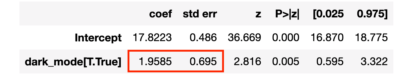
The estimated effect of dark_mode is positive, significant at the 1% level, and very close to the true value of 2!
Conclusion
In this blog post, we have seen how to perform conditional analysis using different approaches. Matching directly matches most similar units in the treatment and control groups. Weighting simply assigns different weights to different observations depending on their probability of receiving the treatment. Regression instead weights observations depending on the conditional treatment variances, giving more weight to observations that have characteristics common to both the treatment and control group.
These procedures are extremely helpful because they can either allow us to estimate causal effects from (very rich) observational data or correct experimental estimates when randomization was not perfect or we have a small sample.
Last but not least, if you want to know more, I strongly recommend this video lecture on propensity scores from Paul Goldsmith-Pinkham which is freely available online.
The whole course is a gem and it is an incredible privilege to have such high-quality material available online for free!
References
[1] P. Rosenbaum, D. Rubin, The central role of the propensity score in observational studies for causal effects (1983), Biometrika.
[2] G. Imbens, K. Hirano, G. Ridder, Efficient Estimation of Average Treatment Effects Using the Estimated Propensity Score (2003), Econometrica.
[3] J. Angrist, J. S. Pischke, Mostly harmless econometrics: An Empiricist’s Companion (2009), Princeton University Press.
Related Articles
- Understanding The Frisch-Waugh-Lovell Theorem
- How to Compare Two or More Distributions
- DAGs and Control Variables
Code
You can find the original Jupyter Notebook here:
Thank you for reading!
I really appreciate it!  If you liked the post and would like to see more, consider following me. I post once a week on topics related to causal inference and data analysis. I try to keep my posts simple but precise, always providing code, examples, and simulations.
Also, a small disclaimer: I write to learn so mistakes are the norm, even though I try my best. Please, when you spot them, let me know. I also appreciate suggestions on new topics!


