YOLO v4: Optimal Speed & Accuracy for object detection
A review of a state-of-the-art model for real-time object detection

You only look once (YOLO) is a family of one-stage object detectors that are fast and accurate. Recently, YOLO v4 paper was released and showed very good results compared to other object detectors.
Update 1: Added a colab demo
Table of contents
Introduction
Most of the modern accurate models require many GPUs for training with a large mini-batch size, and doing this with one GPU makes the training really slow and impractical. YOLO v4 addresses this issue by making an object detector which can be trained on a single GPU with a smaller mini-batch size. This makes it possible to train a super fast and accurate object detector with a single 1080 Ti or 2080 Ti GPU.
YOLO v4 achieves state-of-the-art results at a real time speed on the MS COCO dataset with 43.5 % AP running at 65 FPS on a Tesla V100. Pretty interesting results! To achieve these results, they combine some features such as Weighted-Residual-Connections (WRC), Cross-Stage-Partial-connections (CSP), Cross mini-Batch Normalization (CmBN), Self-adversarial-training (SAT) and Mish-activation, Mosaic data augmentation, DropBlock regularization, and CIoU loss. These are referred to as universal features because they should work well independently from the computer vision tasks, datasets and models. We will talk about these features later.

Note: models that fall in the light-blue area are considered real-time object detectors (+30 FPS)
We can see that EfficientDet D4-D3 achieves better AP than YOLO v4 models, but they run at speed of < 30 FPS on a V100 GPU. On the other hand, YOLO is able to run at a much higher speed (> 60 FPS) with very good accuracy.
General Architecture of an Object Detector
Although YOLO are one-stage detectors, there are also two-stage detectors like R-CNN, fast R-CNN and faster R-CNN which are accurate but slow. We will focus on the former ones. Let's take a look at the main components of a modern one-stage object detector.

Backbone
Models such as ResNet, DenseNet, VGG, etc, are used as feature extractors. They are pre-trained on image classification datasets, like ImageNet, and then fine-tuned on the detection dataset. Turns out that, these networks that produce different levels of features with higher semantics as the network gets deeper (more layers), are useful for latter parts of the object detection network.
Neck
These are extra layers that go in between the backbone and head. They are used to extract different feature maps of different stages of the backbone. The neck part can be for example a FPN[1], PANet[2], Bi-FPN[3], among others. For example, YOLOv3 uses FPN to extract features of different scales from the backbone.
What does a Feature Pyramid Network (FPN)?
Augments a standard convolutional network with a top-down pathway and lateral connections so the network efficiently constructs a rich, multi-scale feature pyramid from a single resolution input image [4]

Each lateral connection merges the feature maps from the bottom-up pathway to the top-down pathway, producing different pyramid levels. Before merging the feature maps, the previous pyramid level is up-sampled by a factor of 2x in FPN[1] so they have the same spatial size. The classification/regression network (the head) is then applied at each each level of the pyramid so that it helps to detect object of different sizes.
This idea of Feature Pyramid Networks can be applied to different backbones models, and as an example, the original FPN[1] paper used ResNets. There are also many modules that integrate FPN in different ways, such as SFAM [7], ASFF [9], and Bi-FPN[3].

Image (a) shows how features are extracted from the backbone in a Single Shot Detector architecture(SSD). The image above shows also three other different types of pyramid networks, but the idea behind them is the same as they help to:
Alleviate the problem arising from scale variation across object instances [3].
ASFF[9] and Bi-FPN[3] are also interesting types of FPNs and show interesting results, but we will skip them here.
Head
This is a network in charge of actually doing the detection part (classification and regression) of bounding boxes. A single output may look like (depending on the implementation): 4 values describing the predicted bounding box (x, y, h, w) and the probability of k classes + 1 (one extra for background). Objected detectors anchor-based, like YOLO, apply the head network to each anchor box. Other popular one-stage detectors, which are anchor-based, are: Single Shot Detector[6] and RetinaNet[4].
Following illustration combines the three modules mentioned above.

Bag of freebies & Bag of specials
The authors of YOLO v4 paper[5] distinguish between two categories of methods that are used to improve the object detector’s accuracy. They analyze different methods in both categories, to achieve a fast operating-speed neural network with good accuracy. These both categories are:
Bag of freebies (BoF):
Methods that can make the object detector receive better accuracy without increasing the inference cost. These methods only change the training strategy or only increase the training cost. [5]
An example of BoF is data augmentation, which increases the generalization ability of the model. To do this we can do photo-metric distortions like: changing the brightness, saturation, contrast and noise or we can do geometric distortion of an image, like rotating it, cropping, etc. These techniques are a clear example of a BoF, and they help the detector accuracy!

Note: for object detection tasks the bounding boxes should also have the same transformations applied
There are other interesting techniques of augmenting the images like CutOut[8] which randomly masks out square regions of input during training. This showed to improve robustness and performance of CNNs. Similarly, Random Erasing[10] selects rectangle regions in an image and erases its pixels with random values.

Other Back of Freebies are the regularization techniques used to avoid over-fitting, like: DropOut, DropConnect and DropBlock[13]. This last one actually shows very good results in CNNs and is used in YOLO v4 backbone.

Dropping activations at random (b) is not good to remove semantic information, because nearby activations contain closely related information. Instead, by dropping continuous regions it can remove certain semantic information (e.g., head or feet) and enforce remaining units to learn other features for classifying input image.
The cost function of the regression network also applies to the category. The traditional thing is to apply Mean Squared error to perform regression on the coordinates.

As stated in the paper, this treats these points as independent variables but doesn’t consider the integrity of the object itself. To improve this, IoU[12] loss has been proposed, which takes into consideration the area of the predicted Bounding Box(BBox) and the ground truth Bounding Box. This idea was improved furthermore by GIoU loss [11] by including the shape and orientation of an object in addition to the coverage area. On the other side, CIoU loss was also introduced and it takes into consideration the overlapping area, the distance between center points and aspect ratio. YOLO v4 uses CIoU loss as the loss for the Bounding Boxes, mainly because it leads to faster convergence and better performance compared to the others mentioned.
Note: one thing that might cause confusion is that although many models use MSE for BBox regression loss, they use IoU as a metric and not as a loss function like mentioned above.
Following illustration compares the same model with different IoU losses:

We can notice CIoU performs better than GIoU. These detections come from Faster R-CNN (Ren et al. 2015) which was trained on the same MS COCO dataset, with GIoU and CIoU losses.
Bag of specials (BoS):
Those plugin modules and post-processing methods that only increase the inference cost by a small amount but can significantly improve the accuracy of object detection [5]
As stated in the paper, this kind of modules/methods usually involve: introducing attention mechanisms(Squeeze-and-Excitation and Spatial Attention Module), enlarging receptive field of model and strengthening feature integration capability, among others.
Common modules that are used to improve the receptive field are SPP, ASPP and RFB (YOLO v4 uses SPP).
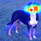
Moreover, attention modules for CNNs are mainly divided in channel wise attention, like Squeeze-and-Excitation (SE)[15], and spatial-wise attention, like Spatial Attention Module (SAM)[16]. A reason why the latter is sometimes preferred, is because SE increases inference speed by a 10% on GPUs, which not desirable. Actually YOLO v4 considers SAM[16] module but not exactly as it was originally published in this paper. Note the following:

Given a feature map F’, the original implementation performed average-pooling and max-pooling operations along the channel axis and then concatenated them. Then a convolution layer is applied (with sigmoid as activation function) to generate an attention map (Ms), which is applied to the original F’.

YOLO v4 modified SAM, on the other hand, doesn’t apply max-pooling and average-pooling, but instead F’ goes through a conv. layer (with sigmoid activation) which then multiplies the original feature map (F’).
Feature Pyramids we discussed early like SFAM[7], ASFF[9] and Bi-FPN[3] also fall in this category of BoS, as do the activation functions. Since ReLU came out, there have been many variants of it, like LReLU, PReLU and ReLU6. Activations like ReLU6 and hard-Swish are specially designed for quantized networks used to make inference on embedded devices, like in the Google Coral Edge TPU.
On the other hand, YOLO v4 uses a lot Mish[14] activation function in the backbone. Take a look at the graph:


Turns out that this activation function shows very promising results. For example, using a Squeeze Excite Network[15] with Mish (on CIFAR-100 dataset) resulted in an increase in Top-1 test accuracy by 0.494% and 1.671% as compared to the same network with Swish and ReLU respectively. [14]
You can check this desmos which contains some other activation functions graphed!
YOLO v4 design
Until now we have discussed methods used improve the model accuracy and different parts of an object detector(backbone, neck, head). Let us now talk about what is used in the new YOLO.
- Backbone: It uses the CSPDarknet53 as the feature-extractor model for the GPU version. For the VPU(Vision Processing Unit) they consider using EfficientNet-lite — MixNet — GhostNet or MobileNetV3. We will focus on the GPU version for now.
The following table shows different considered backbones for GPU version

Certain backbones are more suitable for classification than for detection. For example, CSPDarknet53 showed to be better than CSPResNext50 in terms of detecting objects, and CSPResNext50 better than CSPDarknet53 for image classification. As stated in the paper, a backbone model for object detection requires Higher input network size, for better detection in small objects, and more layers, for a higher receptive field.
- Neck: They use Spatial pyramid pooling (SPP) and Path Aggregation Network (PAN). The latter is not identical to the original PAN, but a modified version which replaces the addition with a concat. Illustration shows this:

Originally in PAN paper, after reducing the size of N4 to have the same spatial size as P5, they add this new down-sized N4 with P5. This is repeated at all levels of 𝑃𝑖+1 and 𝑁𝑖 to produce 𝑁𝑖+1. In YOLO v4 instead of adding 𝑁𝑖 with each 𝑃𝑖+1, they concatenate them (as shown in the image above).

Looking at the SPP module, it basically performs max-pooling over the 19*19*512 feature map with different kernel sizes k = { 5, 9, 13} and ‘same’ padding ( to keep the same spatial size). The four corresponding feature maps get then concatenated to form a 19*19*2048 volume. This increases the neck receptive field, thus improving the model accuracy with negligible increase of inference time.

If you want to visualize different layers used in yolo, like in the image above, I recommend using this tool (either web/desktop version works) and then opening yolov4.cfg with it.
- Head: They use the same as YOLO v3.

These are the heads applied at different scales of the network, for detecting different-size objects. The number of channels is 255 because of (80 classes + 1 for objectness + 4 coordinates) * 3 anchors.
Summary BoF and BoS used
The different modules/methods of BoF and BoS used in the backbone and in the detector of YOLO v4 can be summarized as follows:

Additional Improvements
The authors of the paper introduce a new method of data augmentation called ‘Mosaic’. Basically this combines 4 images of the training dataset in 1 image. By doing this now:
Batch normalization calculates activation statistics from 4 different images on each layer [5]
And so, it greatly reduces the need of selecting a large mini-batch size for training. Checkout following image, showing the new augmentation method.


They also use Self-Adversarial Training (SAT), which operates in 2 forward backward stages. In the 1st stage the neural network alters the original image instead of the network weights. In this way the neural network executes an adversarial attack on itself, altering the original image to create the deception that there is no desired object on the image. In the 2nd stage, the neural network is trained to detect an object on this modified image in the normal way. [5]
Colab Demo
I made a Colab for testing YOLO v4 & tiny version on your own videos. This uses the model trained on MS COCO. You can take a look here
Conclusion
There are many interesting ideas mentioned in this article which could be explained in much more detail, but I hope the main concepts are clear.
Further details can be found in the paper. If you want to train it on your own dataset, check out the official repo.
YOLO v4 achieves state-of-the-art results (43.5% AP) for real-time object detection and is able to run at a speed of 65 FPS on a V100 GPU. If you want less accuracy but much higher FPS, checkout the new Yolo v4 Tiny version at the official repo.
Reference
[1] Feature Pyramid Networks for Object Detection
[2] Path Aggregation Network for Instance Segmentation
[3] EfficientDet: Scalable and Efficient Object Detection
[4] Focal Loss for Dense Object Detection
[5] YOLOv4: Optimal Speed and Accuracy of Object Detection
[6] Single Shot MultiBox Detector (SSD)
[7] A Single-Shot Object Detector based on Multi-Level Feature Pyramid Network
[8] Improved Regularization of Convolutional Neural Networks with Cutout
[9] Learning Spatial Fusion for Single-Shot Object Detection
[10] Random Erasing Data Augmentation
[11] Generalized Intersection over Union: A Metric and A Loss for Bounding Box Regression
[12] UnitBox: An Advanced Object Detection Network
[13] DropBlock: A regularization method for convolutional networks
[14] Mish: A Self Regularized Non-Monotonic Neural Activation Function