Xception: Meet The Xtreme Inception

Intro to Xception
Xception - the Extreme Inception! Sounds cool and Xtreme! But “Why such a name?”, one might wonder! One obvious thing is that the author Francois Chollet (creator of Keras) had been inspired by the Inception architecture. He tells about how he sees the Inception architecture in his abstract, which I’ve quoted below.
We present an interpretation of Inception modules in convolutional neural networks as being an intermediate step in-between regular convolution and the depthwise separable convolution operation
-Francois Chollet in the Xception paper
Another new deep learning term for today, “depthwise separable convolution”. Now, I know that most of you would’ve guessed that it’s some kind of layer. But for those who have never heard it, fret not. I’ve got you covered in this post. We’ll go deeper about what’s a depthwise separable convolution and how it’s used to build the Xception model. And also more on how it builds upon the Inception hypothesis. As always, I’ll try to throw in more illustrations to make the details clear. Let’s dive in!
The Inception Hypothesis
The Inception-style architecture was introduced in the “Going Deeper With Convolution” paper. The authors called the model introduced in the paper as GoogLeNet, which used the Inception blocks. It was a novel and innovative architecture and it still is. Also, it got much attention as many architectures at that time were stacks of more and more layers to increase network capacity. Inception, on the other hand, was more creative and slick!
Rather than just going deeper by simply adding more layers, it also went wide. We’ll see what I mean by “wide” shortly. The Inception blocks take in an input tensor and perform a combination of convolution and pooling in parallel.

For people who have seen or read the Inception papers, you might find that this is not exactly like an Inception block. Yeah, you’re right! I’ve just illustrated it this way so that everybody gets a rough idea of what it does. You can call it “the naive version of inception” as the authors called it.
Now, the actual Inception block is a little bit different in terms of the number of convolutions, their size, and how they’re layered. But this naive illustration conveys what I meant by “wide” before. The block performs convolution with different filter sizes in parallel. And the output tensors are concatenated along the channel dimension i.e stacked one behind the other.
Going a Bit Deeper
Now that you’ve seen the parallel convolution block, I shall go a bit deeper about the block above. The input tensor which is processed by the different convolution would be of shape (BatchSize, Height, Width, Channels). In the Inception block, the input tensor’s channel dimension is reduced using 1x1 convolution before applying 3x3 or 5x5 convolutions. This reduction in channel size is done to reduce the computation when feeding this tensor to the subsequent layers. You can find this concept explained in great detail in the 1x1 convolution article.

Again, this is just another depiction to understand and is not drawn to be the same as the original Inception block. You can give or take some layers, maybe even wider, and make your own version. The input tensor is individually processed by the three convolution towers. And the three separate output tensors are concatenated along the channel dimension. The GoogLeNet uses multiple Inception block and a few other tricks and tweaks to achieve its performance. I believe, now you get the idea of what an Inception block does.
Next, we shall remodel the above block to make it “Xtreme”!
Making it Xtreme
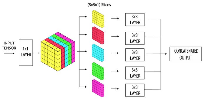
We’ll replace the three separate 1x1 layers in each of the parallel towers, with a single layer. It’ll look something like this.

Rather than just passing on the output of the 1x1 layer to the following 3x3 layers, we’ll slice it and pass each channel separately. Let me illustrate with an example. Say, the output of the 1x1 layer is of shape (1x5x5x5). Let’s not consider the batch dimension and just see it as a (5x5x5) tensor. This is sliced along the channel dimension as shown below and fed separately to the following layers.

Now, each of the slices is passed on to a separate 3x3 layer. This means that each 3x3 block will have to process a tensor of shape (5x5x1). Therefore, there’ll be 5 separate convolution blocks, one for each slice. And each of the convolution blocks will just have a single filter.

This same process scales up to bigger input tensors. If the output of the pointwise convolution is (5x5x100), there’d be 100 convolution blocks each with one filter. And all of their output would be concatenated at last. This way of doing convolution is why it’s named EXTREME as each channel of the input tensor is processed separately.
We have seen enough about the idea of Inception and an Xtreme version of it too. Now, let’s venture further to see what powers the Xception architecture.
Depthwise Separable Convolution: That which powers Xception
The depthwise separable convolution layer is what powers the Xception. And it heavily uses that in its architecture. This type of convolution is similar to the extreme version of the Inception block that we saw above. But differs slightly in its working. Let’s see how!
Consider a typical convolution layer with ten 5x5 filters operating on a (1x10x10x100) tensor. Each of the ten filters is of shape (5x5x100) and slides over the input tensor to produce the output. Each of the 5x5 filters covers the whole channel dimension (the entire 100) as it slides over the input. This means a typical convolution operation encompasses both the spatial (height, width) and the channel dimensions.

If you’re not familiar with convolutions, I suggest you go through How Convolution Works?
A depthwise separable layer has two functional parts that split the job of a conventional convolution layer. The two parts are depthwise convolution and pointwise convolution. We’ll go through them one by one.
Depthwise Convolution
Let’s take an example of a depthwise convolution layer with 3x3 filters that operate on an input tensor of shape (1x5x5x5). Again, let’s lose the batch dimension for simplicity as it doesn’t change anything and consider it as a (5x5x5) tensor. Our depthwise convolution will have five 3x3 filters one for each channel of the input tensor. And each filter will slide spatially through a single channel and generate the output feature map for that channel.
As the number of filters is equal to the number of channels of the input, the output tensor will also have the same number of channels. Let’s not have any zero paddings in the convolution operation and keep the stride as 1.

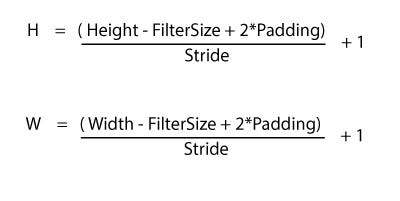
Going by the formula for the output size after convolution, our (5x5x5) will become a (3x3x5) tensor. The illustration below will make the idea clear!

That’s Depthwise Convolution for you! You can see that it’s almost similar to the way we did the Xtreme convolution in the Inception.
Next up, we have to feed this output tensor to a pointwise convolution which performs cross-channel correlation. It simply means that it operates across all the channels of the tensor.
Pointwise Convolution
The pointwise convolution is just another name for a 1x1 convolution. If we ever want to increase or decrease the depth (channel dimension) of a tensor, we can use a pointwise convolution. That’s why it was used in the Inception block to reduce the depth before the 3x3 or 5x5 layers. Here, we’re gonna use it to increase the depth. But how?
The pointwise convolution is just a normal convolution layer with a filter size of one (1x1 filters). Therefore, it doesn’t change the spatial output size after convolution. In our example, the output tensor of the depthwise convolution has a size of (8x8x5). If we apply 50 1x1 filters, we’ll get the output as (8x8x50). And RELU activation is applied in the pointwise convolution layer.
See Pointwise Convolution for more detailed illustrations and its advantages.
Combining the depthwise convolution and pointwise convolution, we get the Depthwise Separable Convolution. Let’s just call it DSC from here.
Differences between DSC and the Xtreme Inception
In the Inception block, first comes the pointwise convolution followed by the 3x3 or 5x5 layer. Since we’d be stacking the DSC blocks on above the other, the order doesn’t matter much. The Inception block applies an activation function on both pointwise and the following convolution layers. But in the DSC, it’s just applied once, after the pointwise convolution.

The Xception author discusses the effect of having activation on both the depthwise and pointwise steps in the DSC. And has observed that learning is faster when there’s no intermediate activation.

Xception Architecture
The author has split the entire Xception Architecture into 14 modules where each module is just a bunch of DSC and pooling layers. The 14 modules are grouped into three groups viz. the entry flow, the middle flow, and the exit flow. And each of the groups has four, eight, and two modules respectively. The final group, i.e the exit flow, can optionally have fully connected layers at the end.
Note: All the DSC layers in the architecture use a filter size of 3x3, stride 1, and “same” padding. And all the MaxPooling layers use a 3x3 kernel and a stride of 2.
Entry Flow of Xception

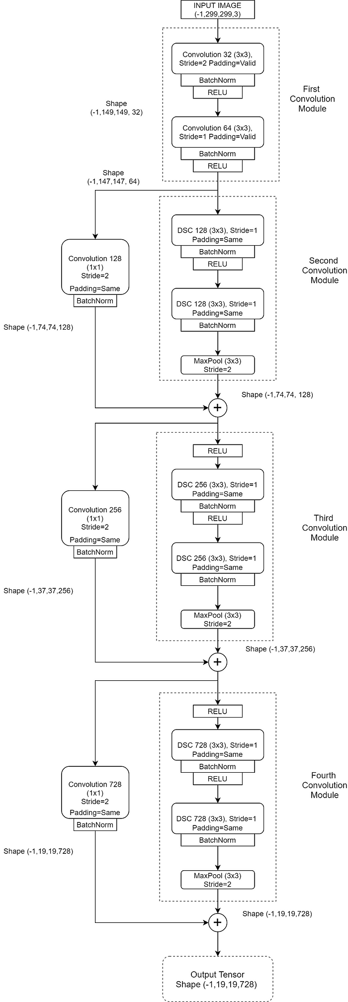
The above illustration is a detailed version of the one given in the Xception paper. Might seem intimidating at first but look again, it’s very simple.
The very first module contains conventional convolution layers and they don’t have any DSC ones. They take input tensors of size (-1, 299, 299, 3). The -1 in the first dimension represents the batch size. A negative -1 just denotes that the batch size can be anything.
And every convolution layer, both conventional and DSC, is followed by a Batch Normalization layer. The convolutions that have a stride of 2 reduces it by almost half. And the output’s shape is shown by the side which is calculated using the convolution formula that we saw before.

Excluding the first module, all the others in the entry flow have residual skip connections. The parallel skip connections have a pointwise convolution layer that gets added to the output from the main path.
Middle Flow of Xception

In the middle flow, there are eight such modules, one after the other. The above module is repeated eight times to form the middle flow. All the 8 modules in the middle flow use a stride of 1 and don’t have any pooling layers. Therefore, the spatial size of the tensor that’s passed from the entry flow remains the same. The channel depth remains the same too as all the middle flow modules have 728 filters. And that’s the same as the input’s depth.
Exit Flow of Xception

The exit flow has just two convolution modules and the second one doesn’t have any skip connection. The second module uses Global Average Pooling, unlike the earlier modules which used Maxpooling. The output vector of the average pooling layer can be fed to a logistic regression layer directly. But we can optionally use intermediate Fully Connected layers too.
To Sum Up
The Xception model contains almost the same number of parameters as the Inception V3 but outperforms Inception V3 by a small margin on the ImageNet dataset. But it beats Inception V3 with a better margin on the JFT image classification dataset (Google’s internal dataset). Performing better with almost the same number of parameters can be attributed to its architecture engineering.


