Wav2Vec 2.0: A Framework for Self-Supervised Learning of Speech Representations

Thoughts and Theory

Model for speech recognition explained

Wav2Vec 2.0 is one of the current state-of-the-art models for Automatic Speech Recognition due to a self-supervised training which is quite a new concept in this field. This way of training allows us to pre-train a model on unlabeled data which is always more accessible. Then, the model can be fine-tuned on a particular dataset for a specific purpose. As the previous works show this way of training is very powerful[4].

Main idea

As presented in the picture below, the model is trained in two phases. The first phase is in a self-supervised mode, which is done using unlabeled data and it aims to achieve the best speech representation possible. You can think about that in a similar way as you think of word embeddings. Word embeddings also aim to achieve the best representation of natural language. The main difference is that Wav2vec 2.0 processes audio instead of text. The second phase of training is supervised fine-tuning, during which labeled data is used to teach the model to predict particular words or phonemes. If you are not familiar with the word ‘phoneme’, you can think about it as the smallest possible unit of sound in a particular language, usually represented by one or two letters.

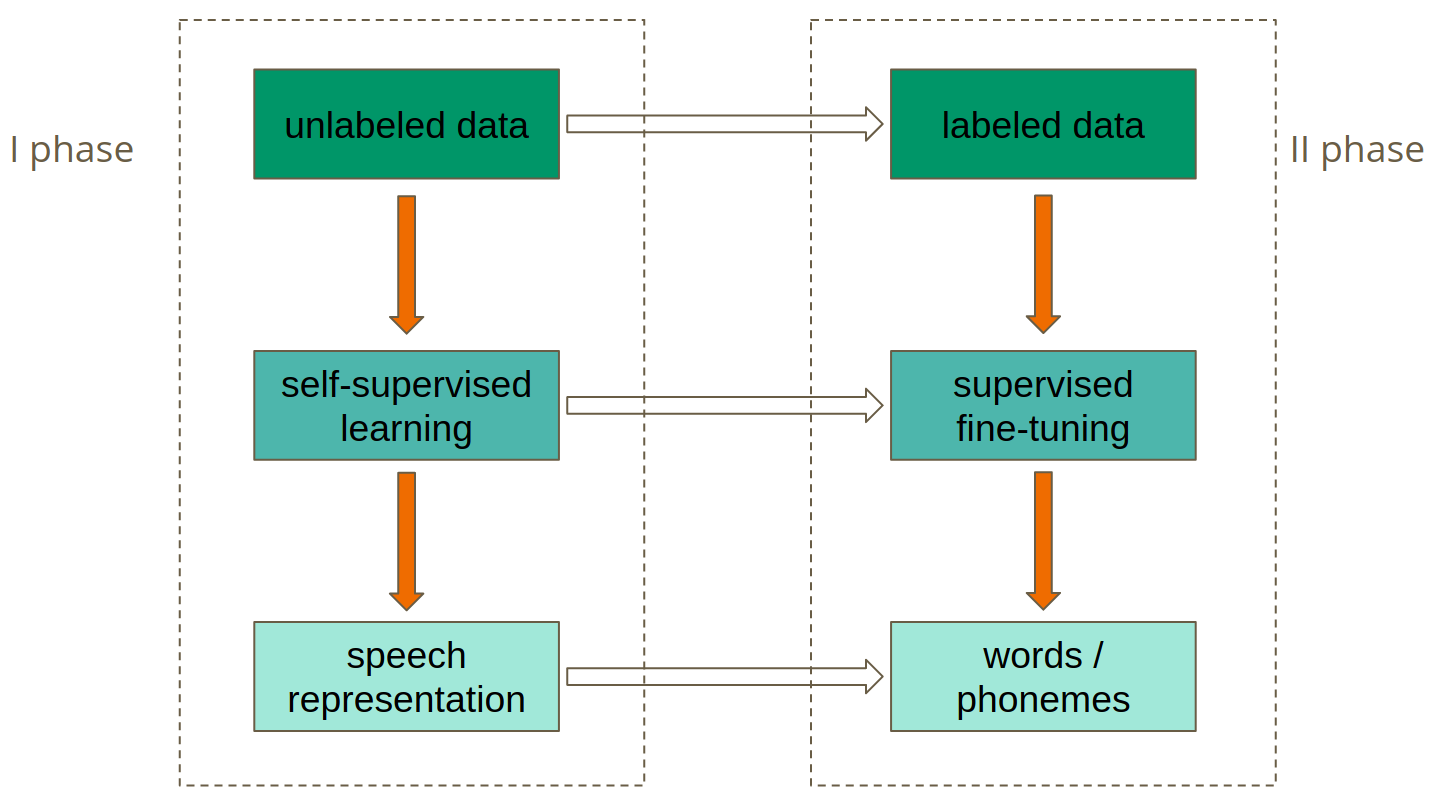
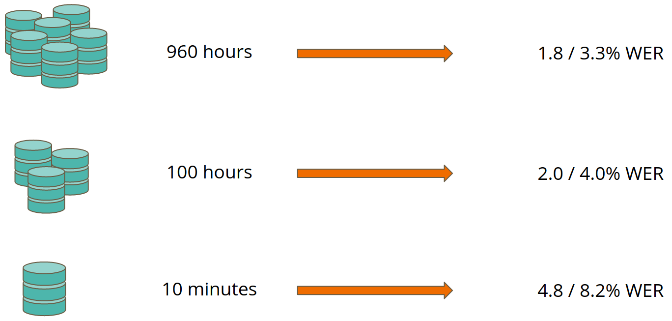
Figure 1. Training phases of Wav2Vec 2.0 (Image by author)

The first phase of training is the main advantage of this model. Learning a very good speech representation enables achieving state-of-the-art results on a small amount of labeled data. For example, the authors of the paper have pre-trained the model on a huge LibriVox dataset. Then, they’ve used the whole Libri Speech dataset for fine-tuning which resulted in 1.8% Word Error Rate (WER) on test-clean subset and 3.3% WER on test-other. Using nearly 10 times less data, allowed to get 2.0% WER on test-clean and 4.0% on test-other. Using only 10 minutes of labeled training data, which is almost no data, resulted in 4.8% / 8.2% WER on test-clean / test-other subsets of Libri Speech. According to Papers With Code, it would have been around the state-of-the-art level in January 2018[5].

Figure 2. Results of Wav2Vec 2.0 (Image by author)

Wav2Vec 2.0 Model Architecture

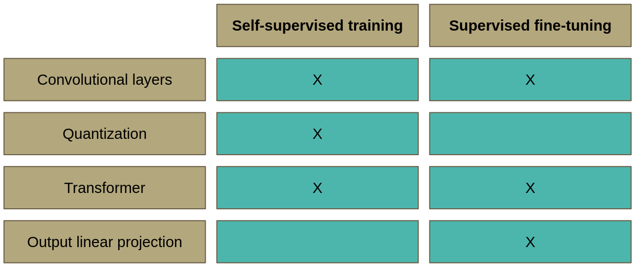
The architecture of the final model used for prediction consists of three main parts:

convolutional layers that process the raw waveform input to get latent representation – Z,
transformer layers, creating contextualised representation – C,
linear projection to output – Y.

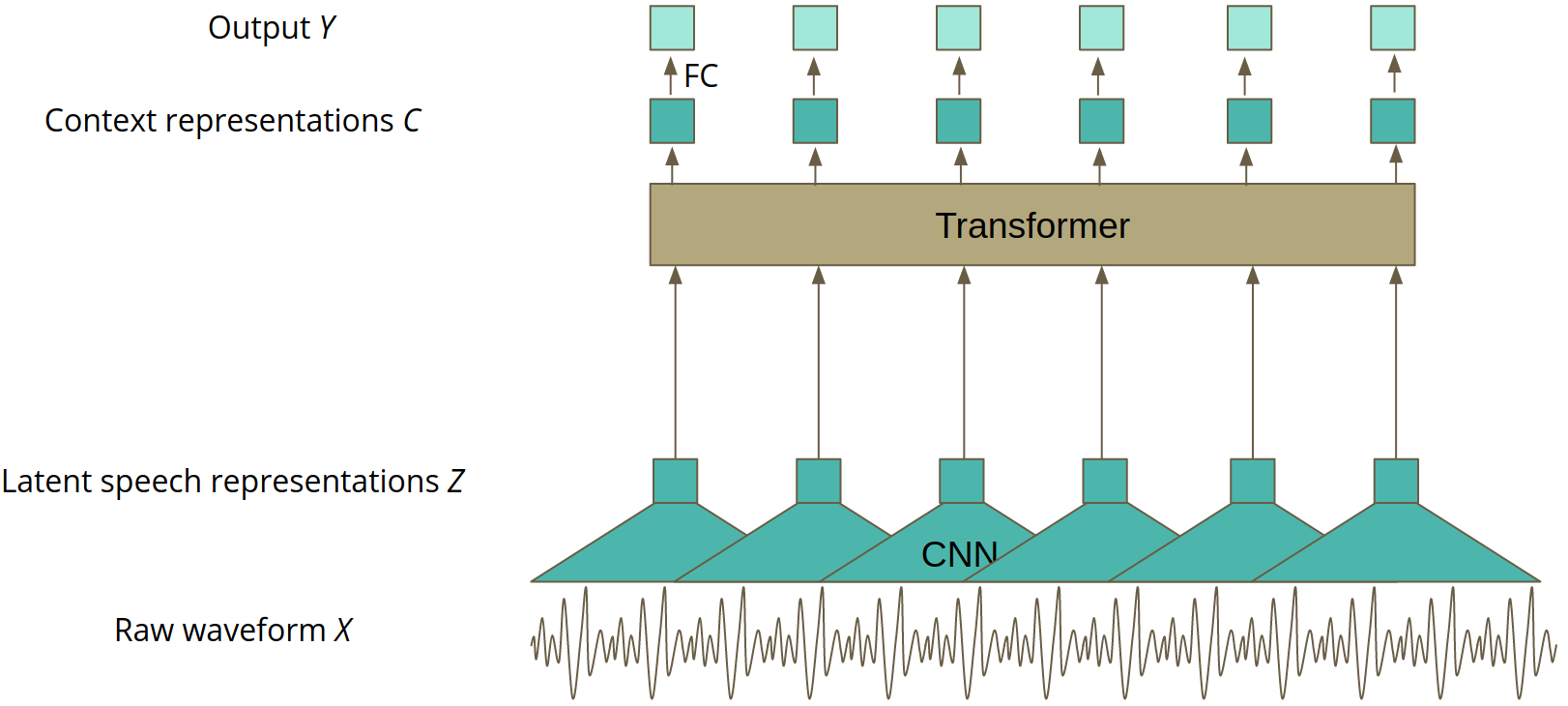
Figure 3. Fine-tuned Wav2Vec 2.0 model architecture (Image by author, based on wav2vec 2.0: A Framework for Self-Supervised Learning of Speech Representations)

That is what the model looks like after final fine-tuning, ready to be developed in a production environment. The whole magic happens during the first phase of training, in the self-supervised mode, when the model looks a little different. The model is trained without the linear projection generating an output prediction.

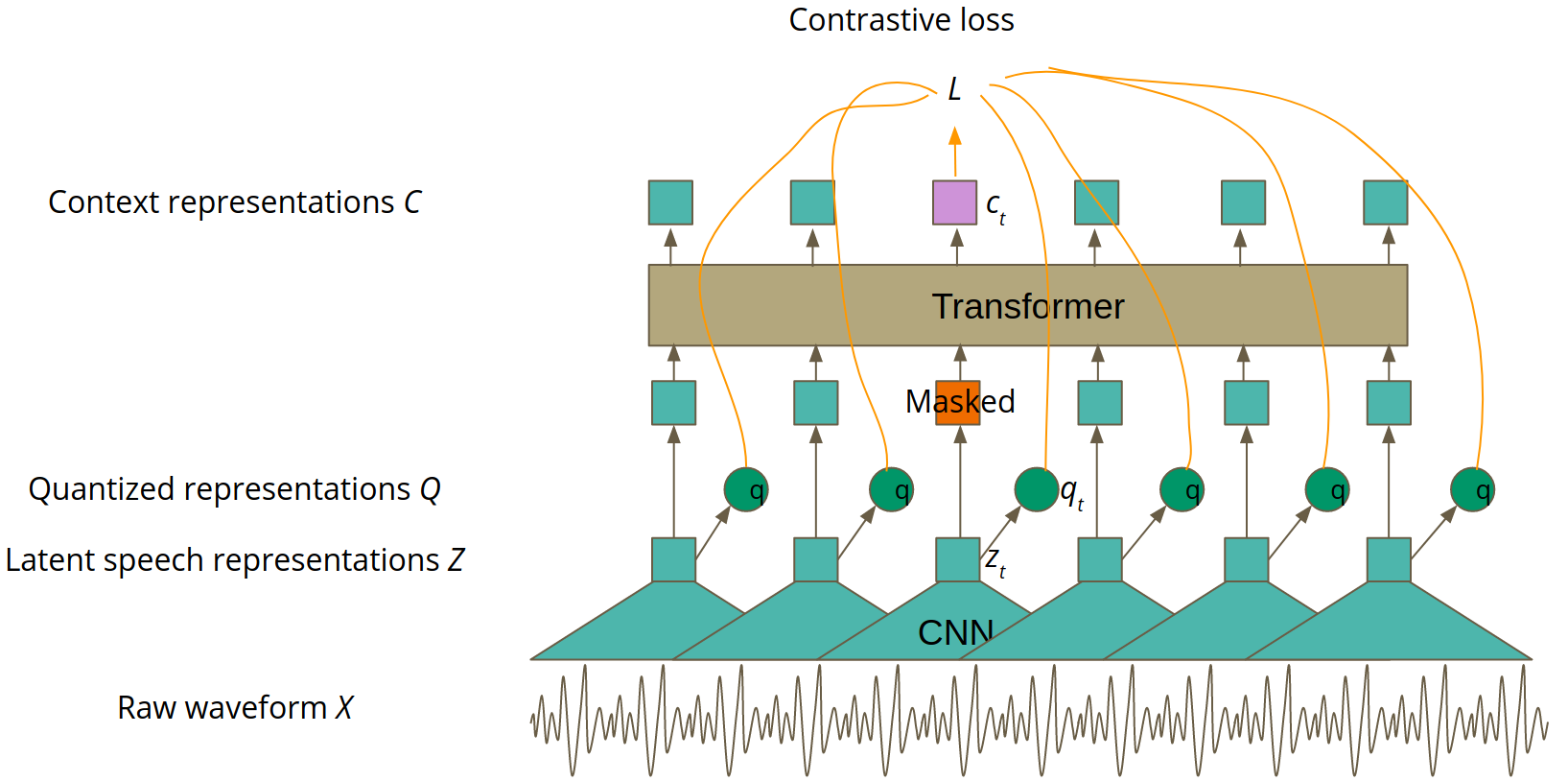
Basically, the speech representation that has been mentioned in the Main idea part of this article corresponds to ‘context representation C‘ in Figure 4. The main idea of pre-training is similar to BERT: part of the transformer’s input is masked and the aim is to guess the masked latent feature vector representation zₜ. However, the authors have improved that simple idea with contrastive learning.

Contrastive learning

Contrastive learning is a concept in which the input is transformed in two different ways. Afterwards, the model is trained to recognise whether two transformations of the input are still the same object. In Wav2Vec 2.0, the transformer layers are the first way of transformation, the second one is made by quantization, which will be explained in the further part of this article. More formally, for a masked latent representation zₜ, we would like to get such a context representation cₜ to be able to guess the correct quantized representation qₜ among other quantized representations. It is important to understand the previous sentence well, so do not hesitate to stop here if you need to The version of Wav2Vec 2.0 used for self-supervised training is presented in Figure 4.

Figure 4. Wav2Vec 2.0 model architecture for self-supervised training (Image by author, based on wav2vec 2.0: A Framework for Self-Supervised Learning of Speech Representations)

To sum up what we’ve learned so far, please take a look at Table 1.

Table 1. Comparison of self-supervised and supervised learning of Wav2Vec 2.0

Quantization

Quantization is a process of converting values from a continuous space into a finite set of values in a discrete space.

But how can we implement this in automatic speech recognition? Let’s assume that one latent speech representation vector zₜ covers two phonemes. The number of phonemes in a language is finite. Moreover, the number of all possible pairs of phonemes is finite. It means they can be perfectly represented by the same latent speech representation. Furthermore, the number of them is finite, so we can create a codebook containing all possible pairs of phonemes. Then, the quantization comes down to choosing the right code word from the codebook. However, you can imagine that the number of all possible sounds is huge. To make it easier to train and use, the authors of Wav2Vec 2.0 created G codebooks, each one consisting of V code words. To create a quantized representation, the best word from every codebook should be selected. Then, the chosen vectors are concatenated and processed with a linear transformation to obtain a quantized representation. The process is presented in Figure 5.

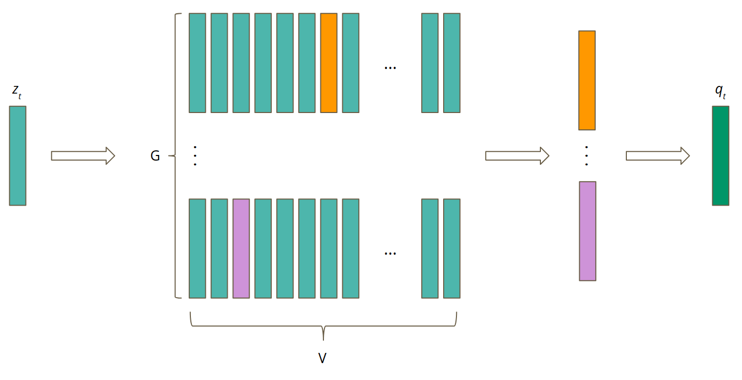
Figure 5. Quantization (Image by author)

How do we choose the best code word from every codebook? The answer is Gumbel softmax:

where:

sim – cosine similarity,
l ϵ ℝᴳˣⱽ – logits calculated from z,
nₖ = -log(-log(uₖ)),
uₖ is sampled from the uniform distribution U(0, 1),
𝜏 – temperature.

Since it’s a classification task, a softmax function seems to be a natural choice for choosing the best code word in every codebook. Why, in our case, is Gumbel softmax better than a normal softmax? It comes with two improvements: randomization and temperature 𝜏. Due to randomization, the model is more willing to choose different code words during training and then to update their weights. It is important, especially in the beginning of training, to prevent using only a subset of codebooks. The temperature is lowered over time from 2 to 0.5, so the impact of randomization is getting smaller with time.

Masking

Let’s dive into the details of masking. It is defined with two hyperparameters: p = 0.065 **** and M = 10 and it is conducted with the following steps:

Take all time steps from the space of latent speech representation Z.
Sample without replacement proportion p of vectors from the previous step.
Chosen time steps are starting indices.
For each index i, consecutive M time steps are masked.

As presented in the next picture, we have sampled two vectors marked with orange colour as starting indices.

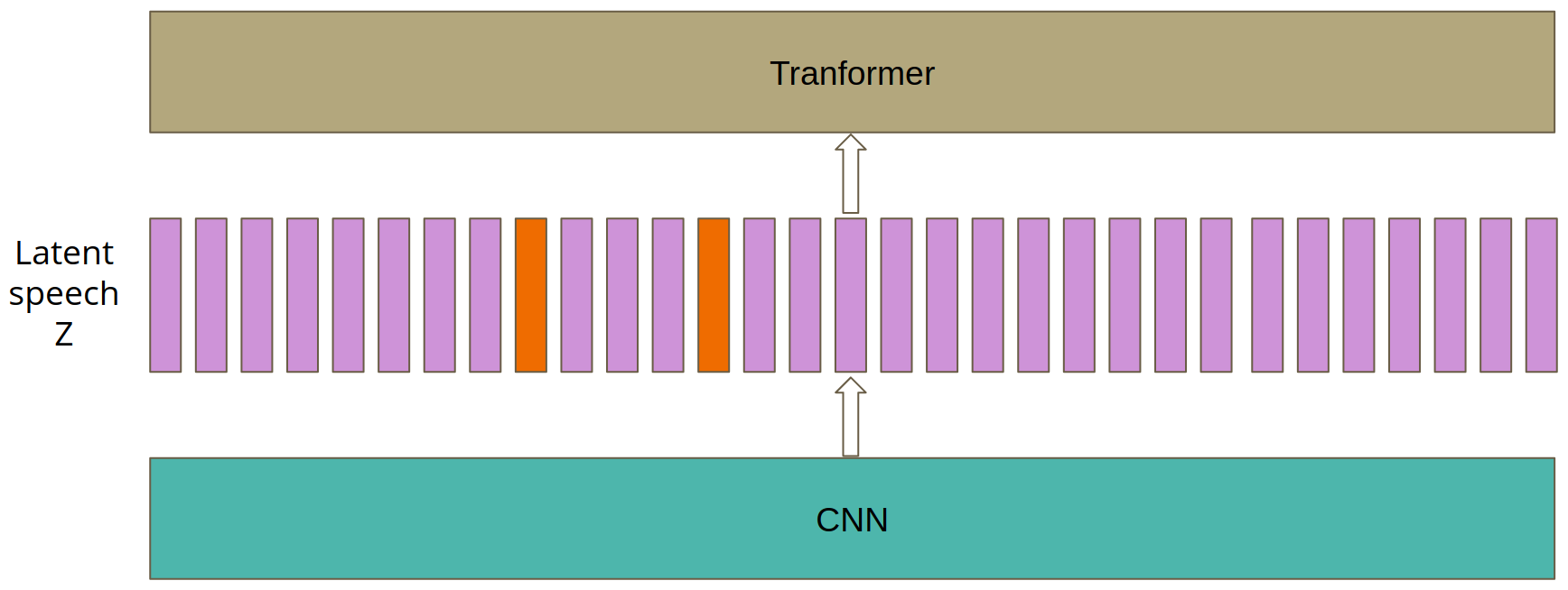
Figure 6. Choosing starting indices for masking (Image by author)

Then, starting from each selected vector, M = 10 consecutive time steps are masked. Spans may overlap, and since the gap between them equals 3 time steps, we mask 14 consecutive time steps.

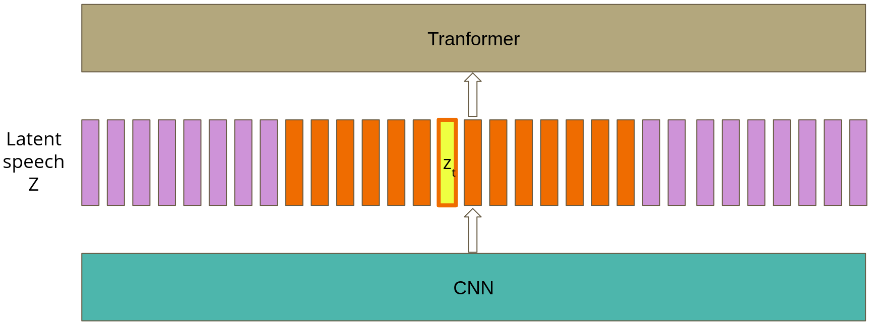
Figure 7. Masking M consecutive time steps (Image by author)

Lastly, the contrastive loss is calculated only for the mask’s central time step.

Training objective

The training objective is a sum of two loss functions: contrastive loss and diversity loss. For now, only the contrastive loss has been mentioned. It is responsible for training the model to predict the correct quantized representation qₜ among K + 1 quantized candidate representations q’ ∈ Qₜ. Set Qₜ consists of target qₜ and K distractors sampled uniformly from other mask time steps.

The letter κ is a temperature which is constant during training. Sim stands for cosine similarity. The main part of function Lₘ is similar to softmax but instead of scores we take cosine similarities between context representation cₜ and quantized representations q. For easier optimization we also put -log on that fraction.

Diversity loss is a kind of regularization technique. The authors have set G=2 codebooks with V=320 code words in every codebook. It theoretically gives 320*320=102400 number of possible quantized representations. However, we do not know if the model will really use all of those possibilities. Otherwise, it will only learn to use, for example, 100 code words from each codebook and it will waste the whole potential of the codebook. That’s why the diversity loss can be useful. It is based on entropy, which can be calculated with the following formula:

where:

x – a possible outcome of discrete random variable 𝒳,
P(x) – probability of event x.

Entropy assumes the maximum value when the data distribution is uniform. In our case, it means that all of the code words are used with the same frequency. With this, we can calculate the entropy of every codebook over the whole batch of training examples to check if the code words are used with the same frequency. Maximization of this entropy will encourage the model to take advantage of all code words. The maximization equals minimization of negative entropy which is the diversity loss.

Fine-tuning

As the fine-tuning phase of Wav2Vec 2.0 does not consist of any groundbreaking discovery, the authors did not pay much attention to this part of their paper. During this stage of training, the quantization is not used. Instead of this, a randomly initialized linear projection layer is added on top of the context representation C. The model then is fine-tuned with standard Connectionist Temporal Classification (CTC) loss and a modified version of SpecAugment which is out of the scope of this article. Interestingly, the authors did not resign from masking because it can still serve as a regularization technique.

Conclusion

Wav2Vec 2.0 uses a self-supervised training approach for Automatic Speech Recognition, which is based on the idea of contrastive learning. Learning speech representation on a huge, raw (unlabeled) dataset reduces the amount of labeled data required for getting satisfying results.

Key takeaways from this article:

Wav2Vec 2.0 takes advantage of self-supervised training,
it uses convolutional layers to preprocess raw waveform and then it applies transformer to enhance the speech representation with context,
its objective is a weighted sum of two loss functions:
contrastive loss,
diversity loss,
quantization is used to create targets in self-supervised learning.

I hope you enjoyed my article and it helped you to understand the idea of Wav2Vec 2.0. For more details, I encourage you to read the original paper[1].

References

[1] A. Baevski, H. Zhou, A. Mohamed and M. Auli, wav2vec 2.0: A Framework for Self-Supervised Learning of Speech Representations (2020), CoRR
[2] A. Kim, The intuition behind Shannon’s Entropy (2018), Towards Data Science
[3] Entropy (information theory), Wikipedia.
[4] J. Devlin, M. Chang, K. Lee, K. Toutanova, BERT: Pre-training of Deep Bidirectional Transformers for Language Understanding _ (2019)_.
[5] Speech Recognition on LibriSpeech test-clean, __ Papers With Code.
![Fig 3D: The architecture of a steerable CNN as described in [3]. Notice the use of the steerable filters in layer 2 coupled together with a G-convolution.](https://towardsdatascience.com/wp-content/uploads/2023/11/0PBKBmh-QW0hhAsXR.png)