Using Machine Learning to Predict Customer Churn

Supervised Machine Learning

Photo by Gertrūda Valasevičiūtė on Unsplash

Introduction

In this article I will walk you through a real business use case for Machine Learning. Often businesses are required to take proactive steps to curtail customer attrition (churn). In the age of big data and machine learning, predicting customer churn has never been more achievable.

I use four machine learning approaches and recommend the best based on performance. The four models I’ve used are: logistic regression, decision tree, random forest classifier, and gradient boosting machine classifier.

To assess model performance base on two criteria: training time and predictive power. AUC is the metric used to measure predictive power because it provides a good measure of a model’s ability to discriminate between customers that churn and those that don’t.

Data

Models are trained on a data set of customers (each identified by a unique customer id). Features are customer attributes in relation to the business. They include the following:

Gender – The customer’s gender as specified on sign-up

Join Date – The date a customer joined

Contact Propensity – The probability a customer will contact customer services

Country ID – An identifier that can be joined on to the country table to get the name of the customer’s current country of residence. The country table is also available for analysis.

The target (or label) is the churn flag, it identifies cases where customers have stopped dealing with the business.

Data Preparation

This is the first step of the machine learning pipeline where some initial exploration, merging of data sources, and data cleaning is conducted.

Merging data: Customer attribute and country data are merged on country ID to bring in the names for the current country of residence.

Duplicates: In the context of the customer data, duplicate observations probably imply erroneous data curation as there should only be a single instance of a customer in the data. There were no duplicate observations found.

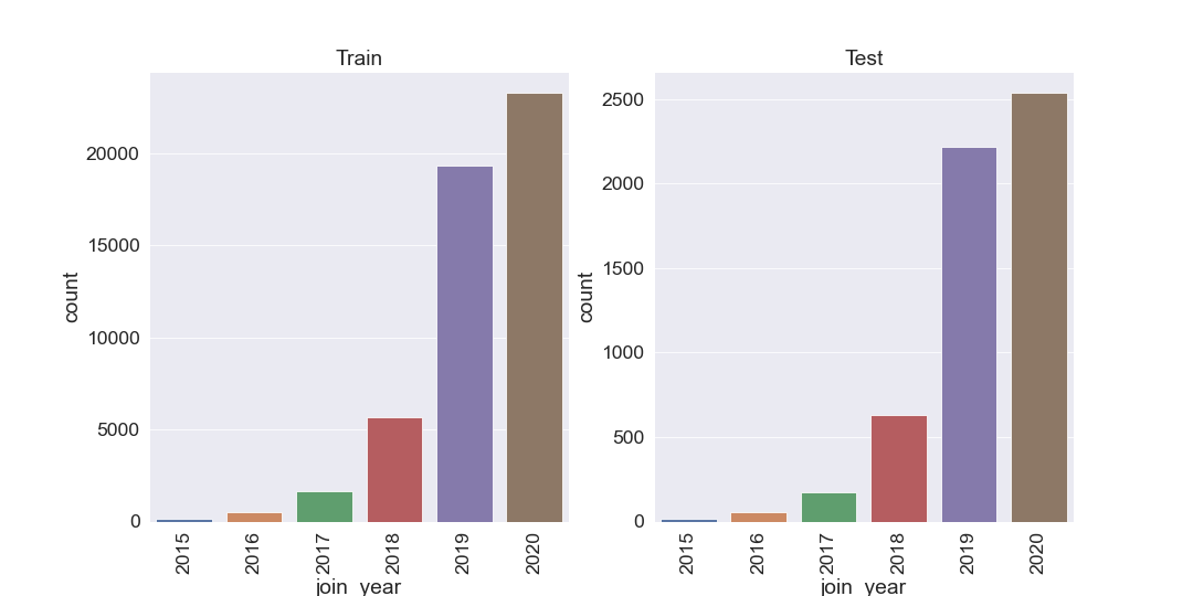
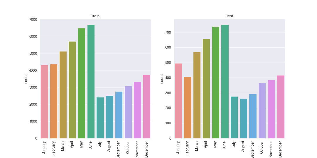
Initial feature engineering: Join date is a datetime feature that has been split out into join month and join year. The split gives the model the opportunity to capture potential seasonal effects on customer churn.

Test & Train: The customer data is split into test and train datasets. Customers having a missing churn flag are allocated to the test set, all other customers are in the train set. The number of unique customers in the test and train data sets are 5,622 and 50,598 respectively.

From this point onwards testing and training data are treated separately to prevent data leakage between the two which could adversely affect machine learning effectiveness.

Missing data: A large volume of missing data will impact modelling down-stream. A simple check for N/A or Null values is performed to ensure there a none in test or train. There were no unexpected missing values.

Exploratory Data Analysis

Initial data exploration reveals some interesting quirks.

Gender: Across both training and testing there are three unique gender categories. Male, female and U (unknown). The Unknown cases account for roughly 5% of all cases across both test and train sets.

There are two possible explanations for the unknown cases. 1) Customers who have chosen not to disclose their gender. 2) Data input or data quality issues leading to loss of information.

It is difficult to say for sure what the split is between the two scenarios is for the unknown cases. I have therefore made a simplifying assumption that unknown cases are people that have chosen not to disclose their gender. On this basis, it is sensible to believe that this group of people might behave differently to those that have chosen to identify. This is my justification for leaving unknown cases within the training data.

Unknown cases are distributed across churn and sticking customers in similar ratios to male and female customers.

Missing & unknown country: In the training data there are a total of 12 customers whose current country of residence is either missing or unknown. This relative tiny subset of the training set is likely due to data input or collection errors. It does not seem likely that a customer can sign-up to the service without explicitly stating their country of residence. Because of this, I will omit these observations from the training data.

Note: If this country of current resident is continually updated, it could be worth while to keep the missing data as it’s own category.

Unusual join dates: In the training data some customers have join dates of 1901 indicating some data quality issues. These observations have been omitted from the analysis.

Very old customer: One customer in the test data had an age of 150. This is almost certainly data input error as the current oldest person in the world is 117. Ridiculous age observations have been corrected by replacing observations with an age greater than 117 with the mean age of customers in their country of residence.

Note: 117 is the age of the oldest living person at the time of writing. This may likely need to be revisited.

Train & Test data: The split of training and test is based on missing churn flags. This makes sense as the objective is to infer the missing churn flags. However, it is sensible to check that the testing population is a representative sample of the training population.

We can visualise this by plotting distributions across our features and comparing them across test and train. Looking at the distributions by eye, the test set does appear to be a subset of the training set which is what we require for effective machine learning.

Current country of residence distribution

One Hot Encoding

Machine learning models interpret numbers not words. Our customer data has categorical variables that must be transformed such that the machine learning models are able to work with them. This is done via one hot encoding.

Modelling

Four machine learning models have been trained following a standard modelling pipeline. A model is selected, and hyper parameters are carefully tuned with a combination of grid search and 5-fold cross validation.

Here’s what the training pipeline looks like in Python. This simple function covers everything up to the results evaluation stage.

	from sklearn.model_selection import GridSearchCV


	def model_pipeline(model, param_grid, x_train, Y_train):

	"""
	Pipeline to train sklearn model using k-fold
	cross validation and grid search

	returns the best model and results for all
	traning runs

	parameters -
	model: an sklearn machine learning model
	param_gird: search space for grid search as dict

	"""

	# Initialisa model with GridSearchCV or just GridSearch

	Tuned_Model = GridSearchCV(
	estimator=model, param_grid=param_grid, scoring="roc_auc", cv=5
	)

	# Fit model & Time the process for training the model
	print("Training Model")
	start_time = time.process_time()

	Tuned_Model.fit(x_train, Y_train)

	print("Finished training model")

	# End of fit time
	print(time.process_time() - start_time, "Seconds")

	return Tuned_Model, pd.DataFrame(Tuned_Model.cv_results_)

view raw MLPipeline.py hosted with

by GitHub

Time and compute constraints have restricted my search space for tuning hyperparameters. However, optimum predictive performance can be approached by following heuristics for tuning:

Logistic Regression: The model has been initialised with L2 regularisation, which reduces the complexity of the model slightly to prevent overfitting.The hyperparameter C is the inverse of the regularisation parameter, it is tuned to find an optimum fit. [1]

	# Model 1: Logistic Regression

	# Train and test a logistic regression model
	from sklearn.linear_model import LogisticRegression

	# Initialise the logistic regression model
	model = LogisticRegression(penalty="l2", solver="liblinear", class_weight="balanced")
	# Set paramters for Grid Search
	param_grid = {"C": [0.001, 0.01, 0.1, 1], "fit_intercept": [True, False]}

	# Train model and get results
	Tuned_LogReg, Results_LogReg = model_pipeline(model, param_grid, x_train, Y_train)

view raw Logreg.py hosted with

by GitHub

Decision Trees: Decision trees are prone to overfitting, tuning the maximum tree depth and the maximum features can circumvent this.

	# Model 2: Decision Tree

	# Train a decision tree
	from sklearn.tree import DecisionTreeClassifier

	# Initialise the decision tree model
	model = DecisionTreeClassifier(criterion="gini", class_weight="balanced")
	# Set paramters for Grid Search
	param_grid = {
	"max_depth": [5, 10, 30],
	"max_features": [0.1, 0.3, 0.7],
	"ccp_alpha": [0, 0.005, 0.01, 0.1],
	}

	# Train model and get results
	Tuned_DecTree, Results_DecTree = model_pipeline(model, param_grid, x_train, Y_train)

view raw DecisionTree.py hosted with

by GitHub

Random Forests: Important hyper parameters to tune are the number of trees and the size of the subset of features to consider at each split [2]. Bootstrapped samples are used to build trees to make the model robust to overfitting.

	# Model 3: Random Forest

	# Train a random forest classifier
	from sklearn.ensemble import RandomForestClassifier

	# Initialise the random forest model
	model = RandomForestClassifier(class_weight="balanced_subsample", bootstrap=True)

	# Set paramters for Grid Search
	param_grid = {
	"n_estimators": [200, 300, 400, 500, 600],
	"max_features": [0.1, 0.3, 0.6],
	}

	# Train model and get results
	Tuned_RandomForest, Results_RandForest = model_pipeline(
	model, param_grid, x_train, Y_train
	)

view raw RandomForestMod.py hosted with

by GitHub

Gradient Boosting Machines: The number of trees, learning rate and the depth of trees are the important hyperparameters to tune [2].

	# Model 4: Gradient Boosting Machines Classifier

	# Train a GBM classifier
	from sklearn.ensemble import GradientBoostingClassifier

	# Initialise the gbm model
	model = GradientBoostingClassifier()

	# Set paramters for Grid Search
	param_grid = {
	"n_estimators": [300],
	"max_depth": [5, 10, 30],
	"learning_rate": [0.01, 0.05, 0.1],
	}

	# Train model and get results
	Tuned_GBM, Results_GBM = model_pipeline(model, param_grid, x_train, Y_train)

view raw GBM.py hosted with

by GitHub

Imbalanced Classes: From our exploratory data analysis, we saw that there is a class imbalance between customers that churn and customers that stick. All models use a class weighting to address this.

Model Evaluation

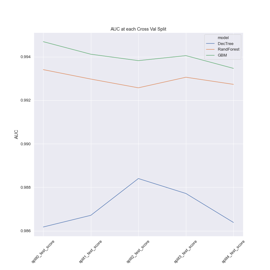
Predictive Power

Predictive performance is evaluated using the AUC. In terms of predictive performance, gradient boosting outperformed all other models with a mean AUC of 0.994. The logistic regression performed poorly yielding a mean AUC of 0.7246.

The decision tree performed well on its best run. However, the variance within its best run and across the search space was the highest of all the models implying some propensity to overfit the training data which is not easy to control for.

Random forest was the second-best performing model in terms of predictive power with a mean AUC of 0.993. However, it was the most robust to overfitting with a variance of 0.000287 between cross validation folds.

Model performance for best hyperparameter space across 5 fold CV

Here’s the Python code used to generate a table with the scores for all the best models.


	def bestmodel(data, modelname):

	"""
	Function geneates best results from each model training
	run.
	data: model result as pandas data frame (from GridSearchCv)
	modelname: name of model used as str

	"""

	bestmodel = data.loc[data.rank_test_score == 1].copy()
	bestmodel["score"] = "AUC"
	keep = [
	"split0_test_score",
	"split1_test_score",
	"split2_test_score",
	"split3_test_score",
	"split4_test_score",
	"score",
	]
	bestmodel_a = bestmodel[keep].copy()
	bestmodel_a.set_index("score", inplace=True)
	bestmodel_b = bestmodel_a.T
	bestmodel_b["model"] = modelname
	bestmodel_c = dict(bestmodel_b)
	return bestmodel_b


	# Set up lists of model results and model names
	data = [Results_DecTree, Results_RandForest, Results_GBM]
	modelname = ["DecTree", "RandForest", "GBM"]
	allbestmodels = pd.DataFrame()

	# Lopp through list of models and model names
	for df, model in zip(data, modelname):
	mod = bestmodel(df, model)

	# concatenate into single table
	allbestmodels = pd.concat([allbestmodels, mod], axis=0)

	# Reset index for plotting
	allbestmodels.reset_index(inplace=True)

view raw Best Models.py hosted with

by GitHub

Here’s the code used to generate the chart above.

	sns.set(font_scale=1.2)
	sns.set_style("darkgrid")
	plt.figure(figsize=(12, 12))
	ax = sns.lineplot(
	y=allbestmodels["AUC"],
	x=allbestmodels["index"],
	hue=allbestmodels["model"],
	ci="sd",
	)
	ax.tick_params(axis="x", labelrotation=45)
	ax.set_title("AUC at each Cross Val Split")
	ax.set_xlabel(" ")
	plt.savefig("ModelEval")
	plt.show()

view raw plotbestmodel.py hosted with

by GitHub

Training Speed

Although gradient boosting was the best performing in terms of predictive power the training speed was slow taking just over half an hour. In contrast, random forest took around half the time for training. Logistic regression and decision trees both trained in under 10 seconds. However, susceptibility to overfitting and poor predictive performance make these unsuitable options for business use.

Best Model

With access to increased compute power, I would recommend gradient boosting. However, random forests deliver excellent predictive performance and a robustness to overfitting that will be important for a production model.

Productionising Models

Ultimately the model will not just sit on your laptop, it will be used at scale by clients and will therefore need to be productionised. Therefore I propose that we should consider the following:

1) Modularise code: Splitting out data ingestion, data cleaning, exploratory data analysis, training and evaluation, and prediction into separate scripts. This will make it much easier to test the scripts and debug the code if required.

2) Customer Data Monitoring: We need to be able to anticipate when model performance could suffer. An easy way to do this is to monitor our current customer population and assess whether it has deviated significantly from past populations.

3) Model Re-Evaluation & re-training: We should look to assess the model’s performance against new data periodically. This could be when we detect data deviations (see point 2) or at a set time frame. If model performance on new data is below our threshold, we will need to re-train the model. Having flexible modelling pipelines will make re-training the model easy to do.

4) Consider Out of Bag score: If using the random forest model, consider using the out of bag validation to speed up the training. Instead of K-fold cross validation, the random forest is validated on the out of bag sample (provided that bootstrapped samples are used to build the trees).

5) Consider training on cloud: If using the gradient boosting, I would consider training the model on a cloud platform such as GCP or AWS to increase the training speed.

6) Expand on training data: Predictive performance could be further increased by including some additional features in the data. Some of these are most frequent corridor and pricing, monthly transactions, referrals, and average transaction amount.