Understanding time complexity with Python examples

Big-O Complexity Chart: http://bigocheatsheet.com/

Nowadays, with all these data we consume and generate every single day, algorithms must be good enough to handle operations in large volumes of data.

In this post, we will understand a little more about time complexity, Big-O notation and why we need to be concerned about it when developing algorithms.

The examples shown in this story were developed in Python, so it will be easier to understand if you have at least the basic knowledge of Python, but this is not a prerequisite.

Let’s start understanding what is computational complexity.

Computational Complexity

Computational complexity is a field from computer science which analyzes algorithms based on the amount resources required for running it. The amount of required resources varies based on the input size, so the complexity is generally expressed as a function of n, where n is the size of the input.

It is important to note that when analyzing an algorithm we can consider the time complexity and space complexity. The space complexity is basically the amount of memory space required to solve a problem in relation to the input size. Even though the space complexity is important when analyzing an algorithm, in this story we will focus only on the time complexity.

Time Complexity

As you’re reading this story right now, you may have an idea about what is time complexity, but to make sure we’re all on the same page, let’s start understanding what time complexity means with a short description from Wikipedia.

In computer science, the time complexity is the computational complexity that describes the amount of time it takes to run an algorithm. Time complexity is commonly estimated by counting the number of elementary operations performed by the algorithm, supposing that each elementary operation takes a fixed amount of time to perform.

When analyzing the time complexity of an algorithm we may find three cases: best-case, average-case and worst-case. Let’s understand what it means.

Suppose we have the following unsorted list [1, 5, 3, 9, 2, 4, 6, 7, 8] and we need to find the index of a value in this list using linear search.

• best-case: this is the complexity of solving the problem for the best input. In our example, the best case would be to search for the value 1. Since this is the first value of the list, it would be found in the first iteration.
• average-case: this is the average complexity of solving the problem. This complexity is defined with respect to the distribution of the values in the input data. Maybe this is not the best example but, based on our sample, we could say that the average-case would be when we’re searching for some value in the “middle” of the list, for example, the value 2.
• worst-case: this is the complexity of solving the problem for the worst input of size n. In our example, the worst-case would be to search for the value 8, which is the last element from the list.

Usually, when describing the time complexity of an algorithm, we are talking about the worst-case.

Ok, but how we describe the time complexity of an algorithm?

We use a mathematical notation called Big-O.

Big-O Notation

Big-O notation, sometimes called “asymptotic notation”, is a mathematical notation that describes the limiting behavior of a function when the argument tends towards a particular value or infinity.

In computer science, Big-O notation is used to classify algorithms according to how their running time or space requirements grow as the input size (n) grows. This notation characterizes functions according to their growth rates: different functions with the same growth rate may be represented using the same O notation.

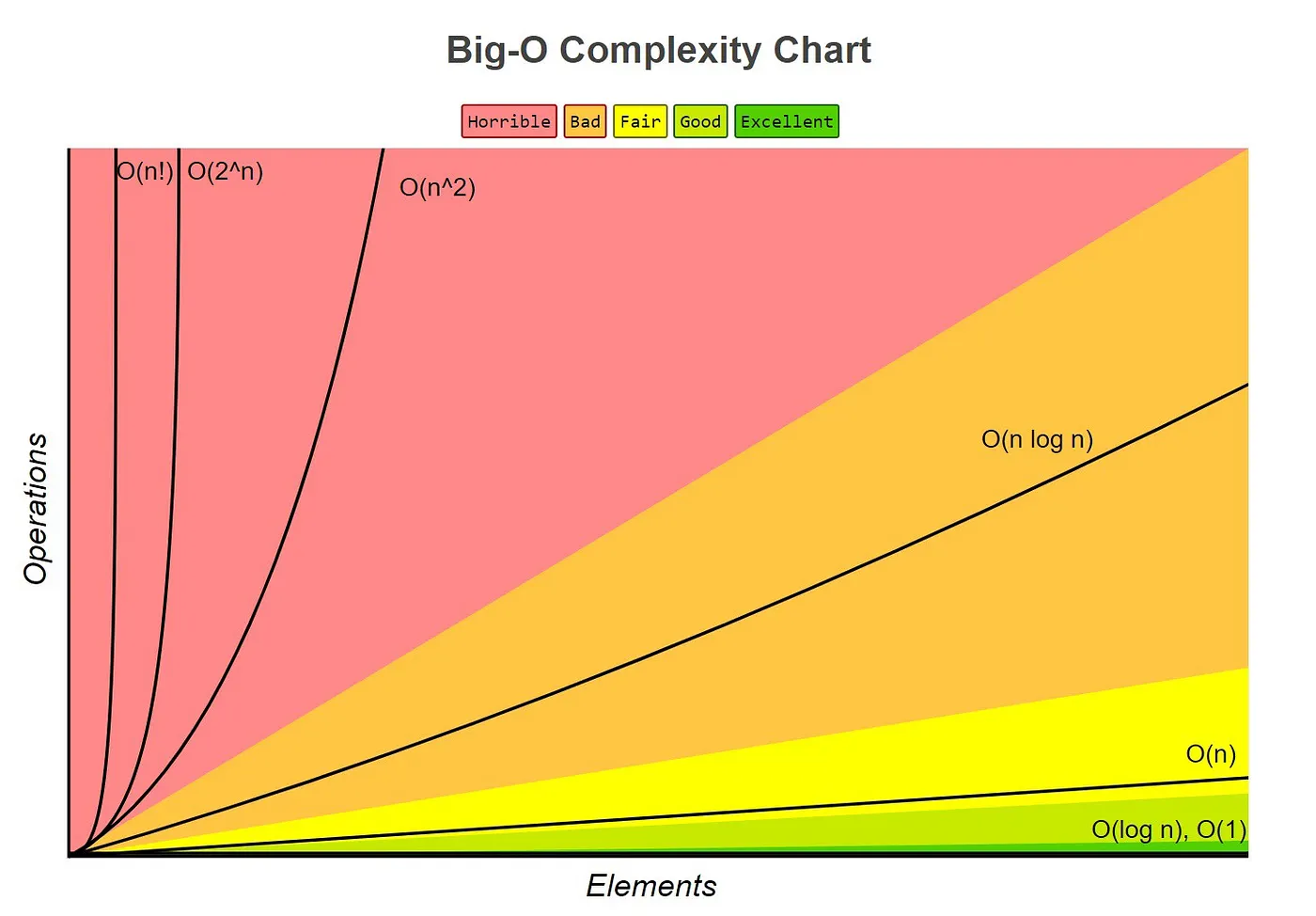
Let’s see some common time complexities described in the Big-O notation.

Table of common time complexities

These are the most common time complexities expressed using the Big-O notation:

╔══════════════════╦═════════════════╗
║       Name       ║ Time Complexity ║
╠══════════════════╬═════════════════╣
║ Constant Time    ║       O(1)      ║
╠══════════════════╬═════════════════╣
║ Logarithmic Time ║     O(log n)    ║
╠══════════════════╬═════════════════╣
║ Linear Time      ║       O(n)      ║
╠══════════════════╬═════════════════╣
║ Quasilinear Time ║    O(n log n)   ║
╠══════════════════╬═════════════════╣
║ Quadratic Time   ║      O(n^2)     ║
╠══════════════════╬═════════════════╣
║ Exponential Time ║      O(2^n)     ║
╠══════════════════╬═════════════════╣
║ Factorial Time   ║       O(n!)     ║
╚══════════════════╩═════════════════╝

Note that we will focus our study in these common time complexities but there are some other time complexities out there which you can study later.

As already said, we generally use the Big-O notation to describe the time complexity of algorithms. There’s a lot of math involved in the formal definition of the notation, but informally we can assume that the Big-O notation gives us the algorithm’s approximate run time in the worst case. When using the Big-O notation, we describe the algorithm’s efficiency based on the increasing size of the input data (n). For example, if the input is a string, the n will be the length of the string. If it is a list, the n will be the length of the list and so on.

Now, let’s go through each one of these common time complexities and see some examples of algorithms. Note that I tried to follow the following approach: present a little description, show a simple and understandable example and show a more complex example (usually from a real-world problem).

Time Complexities

Constant Time — O(1)

An algorithm is said to have a constant time when it is not dependent on the input data (n). No matter the size of the input data, the running time will always be the same. For example:

if a > b:
    return True
else:
    return False

Now, let’s take a look at the function get_first which returns the first element of a list:

def get_first(data):
    return data[0]
    
if __name__ == '__main__':
    data = [1, 2, 9, 8, 3, 4, 7, 6, 5]
    print(get_first(data))

Independently of the input data size, it will always have the same running time since it only gets the first value from the list.

An algorithm with constant time complexity is excellent since we don’t need to worry about the input size.

Logarithmic Time — O(log n)

An algorithm is said to have a logarithmic time complexity when it reduces the size of the input data in each step (it don’t need to look at all values of the input data), for example:

for index in range(0, len(data), 3):
    print(data[index])

Algorithms with logarithmic time complexity are commonly found in operations on binary trees or when using binary search. Let’s take a look at the example of a binary search, where we need to find the position of an element in a sorted list:

def binary_search(data, value):
    n = len(data)
    left = 0
    right = n - 1
    while left <= right:
        middle = (left + right) // 2
        if value < data[middle]:
            right = middle - 1
        elif value > data[middle]:
            left = middle + 1
        else:
            return middle
    raise ValueError('Value is not in the list')
    
if __name__ == '__main__':
    data = [1, 2, 3, 4, 5, 6, 7, 8, 9]
    print(binary_search(data, 8))

Steps of the binary search:

• Calculate the middle of the list.
• If the searched value is lower than the value in the middle of the list, set a new right bounder.
• If the searched value is higher than the value in the middle of the list, set a new left bounder.
• If the search value is equal to the value in the middle of the list, return the middle (the index).
• Repeat the steps above until the value is found or the left bounder is equal or higher the right bounder.

It is important to understand that an algorithm that must access all elements of its input data cannot take logarithmic time, as the time taken for reading input of size n is of the order of n.

Linear Time — O(n)

An algorithm is said to have a linear time complexity when the running time increases at most linearly with the size of the input data. This is the best possible time complexity when the algorithm must examine all values in the input data. For example:

for value in data:
    print(value)

Let’s take a look at the example of a linear search, where we need to find the position of an element in an unsorted list:

def linear_search(data, value):
    for index in range(len(data)):
        if value == data[index]:
            return index
    raise ValueError('Value not found in the list')
    
if __name__ == '__main__':
    data = [1, 2, 9, 8, 3, 4, 7, 6, 5]
    print(linear_search(data, 7))

Note that in this example, we need to look at all values in the list to find the value we are looking for.

Quasilinear Time — O(n log n)

An algorithm is said to have a quasilinear time complexity when each operation in the input data have a logarithm time complexity. It is commonly seen in sorting algorithms (e.g. mergesort, timsort, heapsort).

For example: for each value in the data1 (O(n)) use the binary search (O(log n)) to search the same value in data2.

for value in data1:
    result.append(binary_search(data2, value))

Another, more complex example, can be found in the Mergesort algorithm. Mergesort is an efficient, general-purpose, comparison-based sorting algorithm which has quasilinear time complexity, let’s see an example:

def merge_sort(data):
    if len(data) <= 1:
        return
    
    mid = len(data) // 2
    left_data = data[:mid]
    right_data = data[mid:]
    
    merge_sort(left_data)
    merge_sort(right_data)
    
    left_index = 0
    right_index = 0
    data_index = 0
    
    while left_index < len(left_data) and right_index < len(right_data):
        if left_data[left_index] < right_data[right_index]:
            data[data_index] = left_data[left_index]
            left_index += 1
        else:
            data[data_index] = right_data[right_index]
            right_index += 1
        data_index += 1
    
    if left_index < len(left_data):
        del data[data_index:]
        data += left_data[left_index:]
    elif right_index < len(right_data):
        del data[data_index:]
        data += right_data[right_index:]
    
if __name__ == '__main__':
    data = [9, 1, 7, 6, 2, 8, 5, 3, 4, 0]
    merge_sort(data)
    print(data)

The following image exemplifies the steps taken by the mergesort algorithm.

Mergesort example: https://en.wikipedia.org/wiki/Merge_sort

Note that in this example the sorting is being performed in-place.

Quadratic Time — O(n²)

An algorithm is said to have a quadratic time complexity when it needs to perform a linear time operation for each value in the input data, for example:

for x in data:
    for y in data:
        print(x, y)

Bubble sort is a great example of quadratic time complexity since for each value it needs to compare to all other values in the list, let’s see an example:

def bubble_sort(data):
    swapped = True
    while swapped:
        swapped = False
        for i in range(len(data)-1):
            if data[i] > data[i+1]:
                data[i], data[i+1] = data[i+1], data[i]
                swapped = True
    
if __name__ == '__main__':
    data = [9, 1, 7, 6, 2, 8, 5, 3, 4, 0]
    bubble_sort(data)
    print(data)

Exponential Time — O(2^n)

An algorithm is said to have an exponential time complexity when the growth doubles with each addition to the input data set. This kind of time complexity is usually seen in brute-force algorithms.

As exemplified by Vicky Lai:

In cryptography, a brute-force attack may systematically check all possible elements of a password by iterating through subsets. Using an exponential algorithm to do this, it becomes incredibly resource-expensive to brute-force crack a long password versus a shorter one. This is one reason that a long password is considered more secure than a shorter one.

Another example of an exponential time algorithm is the recursive calculation of Fibonacci numbers:

def fibonacci(n):
    if n <= 1:
        return n
    return fibonacci(n-1) + fibonacci(n-2)

If you don’t know what a recursive function is, let’s clarify it quickly: a recursive function may be described as a function that calls itself in specific conditions. As you may have noticed, the time complexity of recursive functions is a little harder to define since it depends on how many times the function is called and the time complexity of a single function call.

It makes more sense when we look at the recursion tree. The following recursion tree was generated by the Fibonacci algorithm using n = 4:

Recursion tree of Fibonacci(4): https://visualgo.net/bn/recursion

Note that it will call itself until it reaches the leaves. When reaching the leaves it returns the value itself.

Now, look how the recursion tree grows just increasing the n to 6:

Recursion tree of Fibonacci(6): https://visualgo.net/bn/recursion

You can find a more complete explanation about the time complexity of the recursive Fibonacci algorithm here on StackOverflow.

Factorial — O(n!)

An algorithm is said to have a factorial time complexity when it grows in a factorial way based on the size of the input data, for example:

2! = 2 x 1 = 2
3! = 3 x 2 x 1 = 6
4! = 4 x 3 x 2 x 1 = 24
5! = 5 x 4 x 3 x 2 x 1 = 120
6! = 6 x 5 x 4 x 3 x 2 x 1 = 720
7! = 7 x 6 x 5 x 4 x 3 x 2 x 1 = 5.040
8! = 8 x 7 x 6 x 5 x 4 x 3 x 2 x 1 = 40.320

As you may see it grows very fast, even for a small size input.

A great example of an algorithm which has a factorial time complexity is the Heap’s algorithm, which is used for generating all possible permutations of n objects.

According to Wikipedia:

Heap found a systematic method for choosing at each step a pair of elements to switch, in order to produce every possible permutation of these elements exactly once.

Let’s take a look at the example:

def heap_permutation(data, n):
    if n == 1:
        print(data)
        return
    
    for i in range(n):
        heap_permutation(data, n - 1)
        if n % 2 == 0:
            data[i], data[n-1] = data[n-1], data[i]
        else:
            data[0], data[n-1] = data[n-1], data[0]
    
if __name__ == '__main__':
    data = [1, 2, 3]
    heap_permutation(data, len(data))

The result will be:

[1, 2, 3]
[2, 1, 3]
[3, 1, 2]
[1, 3, 2]
[2, 3, 1]
[3, 2, 1]

Note that it will grow in a factorial way, based on the size of the input data, so we can say the algorithm has factorial time complexity O(n!).

Another great example is the Travelling Salesman Problem.

Important Notes

It is important to note that when analyzing the time complexity of an algorithm with several operations we need to describe the algorithm based on the largest complexity among all operations. For example:

def my_function(data):
    first_element = data[0]
    
    for value in data:
        print(value)
    
    for x in data:
        for y in data:
            print(x, y)

Even that the operations in ‘my_function’ don’t make sense we can see that it has multiple time complexities: O(1) + O(n) + O(n²). So, when increasing the size of the input data, the bottleneck of this algorithm will be the operation that takes O(n²). Based on this, we can describe the time complexity of this algorithm as O(n²).

Big-O Cheat Sheet

To make your life easier, here you can find a sheet with the time complexity of the operations in the most common data structures.

Common Data Structure Operations: http://bigocheatsheet.com/

Here is another sheet with the time complexity of the most common sorting algorithms.

Array Sorting Algorithms: http://bigocheatsheet.com/

Why it is important to know all of this?

If after reading all this story you still have some doubts about the importance of knowing time complexity and the Big-O notation, let’s clarify some points.

Even when working with modern languages, like Python, which provides built-in functions, like sorting algorithms, someday you will probably need to implement an algorithm to perform some kind of operation in a certain amount of data. By studying time complexity you will understand the important concept of efficiency and will be able to find bottlenecks in your code which should be improved, mainly when working with huge data sets.

Besides that, if you plan to apply to a software engineer position in a big company like Google, Facebook, Twitter, and Amazon you will need to be prepared to answer questions about time complexity using the Big-O notation.

Final Notes

Thanks for reading this story. I hope you have learned a little more about time complexity and the Big-O notation. If you enjoyed it, please give it a clap and share it. If you have any doubt or suggestion feel free to comment or send me an email. Also, feel free to follow me on Twitter, Linkedin, and Github.

References

• Computational complexity: https://en.wikipedia.org/wiki/Computational_complexity
• Big-O notation: https://en.wikipedia.org/wiki/Big_O_notation
• Time complexity: https://en.wikipedia.org/wiki/Time_complexity
• Big-O Cheat Sheet: http://bigocheatsheet.com/
• A coffee-break introduction to time complexity of algorithms: https://vickylai.com/verbose/a-coffee-break-introduction-to-time-complexity-of-algorithms/