In this post, we’ll walk through the basic concepts , properties, and practical values of Normal distribution. If you want to discuss anything or find an error, please email me at Lvqingchuan@gmail.com 
Warm-up
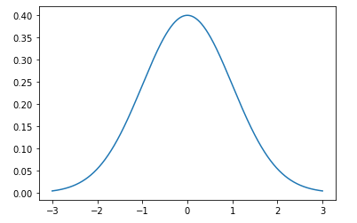
Before getting started, I want you to take a close look at the above diagram. This depicts the density of 10,000 random samples drawn from standard Normal Distribution N(0, 1). What do you see here? This is a fairly symmetric graph with most data points centering around the mean 0. The further from the mean, the less many data points there are. Data points within twice of variance distance from the mean almost cover all data.
Later in this post, we will see the shape of a bell and the distance from the mean lead to important properties of Normal Distribution in general.
Side Bar
We will use the term "random variable" and "standard deviation" in this post. Here’s a brief review:
- A random variable is identically and independently distributed
- Standard deviation, σ, is the square root of variance. Standard Error, s, is the standard deviation divided by the square root of a sample size, σ/sqrt(n).
Basic Concept
The formula of Normal distribution is always given in math and statistic exams. I’m never a fan of memorizing formulas, but this formula is indeed not a hard one to interpret. For an independently and identically distributed variable x, we say x follows normal distribution if the probability density function (pdf.) of x can be written as:

Forget about the first fraction on the left. It just ensures the integral of this probability density function equals to 1. This is one of fundamental properties of being a probability function. Looking into the fraction inside the exponential function, you figure out it’s actually:

Again, forget about the fraction of 1/2 on the left. It just ensures the square of the right part will be cancelled out when you take the first order derivative of the above expression (Remember? The derivative of exp(f(x)) is f'(x)exp(f(x))). Why do we want to take derivatives? Because we want to find the local maxima! To ensure the local/global maxima is at the population mean, we have (x minus population mean) on the numerator; to ensure the curve of the distribution of x is bell-shaped (increases first, then decreases), we have the negative sign in front of 1/2. Besides, thinking again what’s been squared and relevant distributions, you will figure out that (more in the Properties section):

What does chi-square distribution of degree 1 have anything to do here? Remember the graph of chi-square(1):
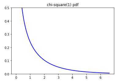
Chi-square(1) is convenient here, as this distribution ensures the increase/decrease rate of probability dense function is smaller as x differs more from the population mean – Bell curve again (BAM!).
Properties
- Linear combination. Combining two normally distributed random variables together, you’ll get a normally distributed random variable again, with different parameters though:

Proving the above statement with a "delicate" probability density function will be a pain. However, you could attack it with characteristic function. Try it yourself, then check this Wikipedia page for an answer. Once the case of two random variables is clear, we could easily generalize it to the case of many (k) random variables by induction.
- Linear transformation. The linear transformation of a normally distributed random variable is still a normally distributed random variable:

The proof of this statement is again by characteristic function. I give the proof of 1-d case as below. You could upgrade it to matrix version on your own.

The only trick in the above proof is letting s = at.
- 68–95–99.7 Rule. This is not an accurate picture of the standard deviation of normal distribution. However, it works quite well in practical estimation. It says when x~N(μ, σ²):

This is just an approximation by looking at the values of cumulative function (z-score) of Normal distribution. Here’s a graph illustration:

Practical Values
- Central Limit Theorem. This famous theorem tells you the distribution of the sample mean of a sufficiently large sample from a population with overall mean μ and variance σ² is N(μ, σ²/n), no matter what the distribution of the population is:

In other words, when you take almost infinitely many samples with replacement repetitively, the sample mean from each batch of your samples will follow normal distribution. ̶I̶ ̶d̶o̶n̶’̶t̶ ̶h̶a̶v̶e̶ ̶a̶n̶ ̶i̶n̶t̶u̶i̶t̶i̶v̶e̶ ̶e̶x̶p̶l̶a̶n̶a̶t̶i̶o̶n̶ ̶a̶b̶o̶u̶t̶ ̶i̶t̶ ̶(̶N̶o̶r̶m̶a̶l̶ ̶d̶i̶s̶t̶r̶i̶b̶u̶t̶i̶o̶n̶ ̶i̶s̶ ̶t̶h̶e̶ ̶o̶n̶e̶ ̶m̶a̶g̶i̶c̶a̶l̶ ̶u̶n̶d̶e̶r̶l̶y̶i̶n̶g̶ ̶p̶o̶w̶e̶r̶?̶ ̶)̶, ̶a̶l̶t̶h̶o̶u̶g̶h̶ this theorem can be proved using characteristic function and Taylor’s Theorem (see this Wikipedia page for reference) theoretically. Update 20220604: an intuitive explanation is throwing dices. When you throw two dices (1–6 on each side) in a row for many times, and compute the sums of two dices each time, you will get a lot more 6–9 than the maximum 12 or the minimum 2. This is because it’s much easier to get median values, such as 1+6, 2+5, 3+4, then to get extreme values, such 6+6.
Central Limit Theorem helps satisfy assumptions about normal distribution with a sufficiently large sample size. Two common examples:
A). T-test and z-test. These tests are very popular in Hypothesis testing and AB testing. In the simplest case, they compare two population mean according to sample Statistics. One necessary condition is the normal distribution of sample mean in each group. Another necessary condition is the normal distribution of observations used to compute standard error in each group. With these two conditions, we’ll be able to construct a test statistic following t-distribution or standard normal distribution. Central Limit Theorem makes your life easy by making these two conditions satisfied as long as you have a very large sample size.
On a side note, almost all the application of t-statistics, such as constructing Confidence Interval of population mean, needs a fairly large sample size, because Central Limit Theorem guarantees you the normal distribution of sample means in each group then.
B). Linear regression. If you want unbiased coefficient estimators with the smallest variance, you need residual terms to follow normally distribution, according to Gauss-Markov Theorem. However, this is not a must-have assumption to get unbiased coefficient estimators. I wrote a post to explain different assumptions of linear regression before: Understanding Linear Regression Assumptions.
- Log transformation. If you plan to use linear regression models, and your label is of the log-normal shape (right skewed), you probably want to apply log transformation to your data. Below is the visualization of labels before and after transformation in my Iowa House Prediction Project:


There are two purposes of using log transformation:
A). Improve the performance of models that are sensitive to skewness, such as Regression Random Forest and Linear Regression. Regression Random Forest uses the average of output of all the trees, and could be far off when there’s an outlier in labels. Similarly, Linear Regression is indeed predicting the conditional expectation of labels. I wrote about Implementing Random Forest and Understanding Linear Regression Assumptions before.
B). Obtain the properties of normal distribution for this transformed variable, such as additivity (linear combination in the Properties section) and linearity (linear transformation in the Properties section). In other words, if you have percentage increase (2%) on the original scale, you will get an additive increase ($20) with the transformed data. This is particularly useful when the scale of your original data varies a lot – 2% increase of $100 is quite different from 2% increase of $1 million. With the log transformation, you will have a much more straightforward view on your data.
As you may have realized, log transformation comes with a price. When you only want to reduce the right-skewness in a linear model, you have to admit that the interpretation of coefficients change from multiplicity (2%) to additivity ($20). Such a change doesn’t make sense in all contexts, especially when your original data was indeed using additive scales.
Besides, if you perform transformation on dependent variables, t-statistic and p-value will change in hypothesis testing. This is not difficult to understand. Log transformation changes standard deviation of data and thus affect t-statistic and p-value, without a certain pattern (could be inflating or deflating). So shall we use the test statistic and p-value when data is log transformed? Mostly yes! As long as your purpose is making data more normal (less skewed) and your log transformation achieves this purpose, there’s no reason for doubting the validity of test statistic or p-value, although they probably will be different from what you get from non-transformed data. However, when you perform log transformation only to make modeling results more interpretable, you don’t want to mess up with hypothesis testing without checking the distribution of transformed data. In the extreme case, when your original data is left skewed, performing log transformation will make data even more left skewed. This makes one of assumptions of t-test, sample mean follows normal distribution, difficult to satisfy. Therefore, test statistic and p-value in this case could be biased.