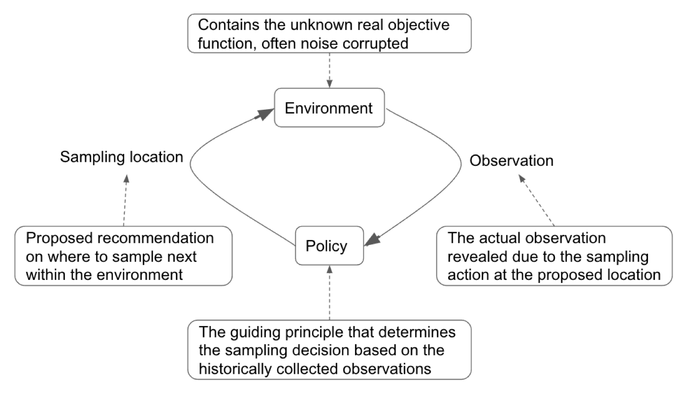
Understanding Bayesian Inference in Bayesian Optimization

Bayesian optimization is an area that studies optimization problems using the Bayesian approach. Optimization aims at locating the optimal objective value (i.e., a global maximum or minimum) of all possible values or the corresponding location of the optimum in the environment. The search process starts at a specific location and follows a particular policy to iteratively guide the following sampling location, collect the corresponding observation, and refresh the policy.

The overall bayesian optimization process. The policy digests the historical observations and proposes the new sampling location, and the environment governs how the (possibly noise corrupted) observation at the newly proposed location is revealed to the policy. Our goal is to learn an efficient and effective policy that could navigate towards the global optimum as quickly as possible. Image by the author.

The objective function

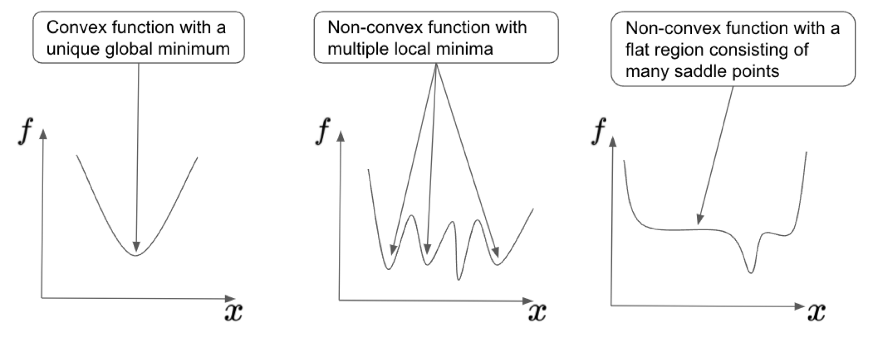
For Bayesian optimization, the specific type of objective function typically bears the following attributes:

We do not have access to the explicit expression of the objective function, making it a "black box" function. This means that we can only interact with the environment, i.e., the objective function, to perform a functional evaluation by sampling at a specific location.
The returned value by probing at a specific location is often corrupted by noise and does not represent the true value of the objective function at that location. Due to the indirect evaluation of its actual value, we need to account for such noise embedded in the actual observations from the environment.
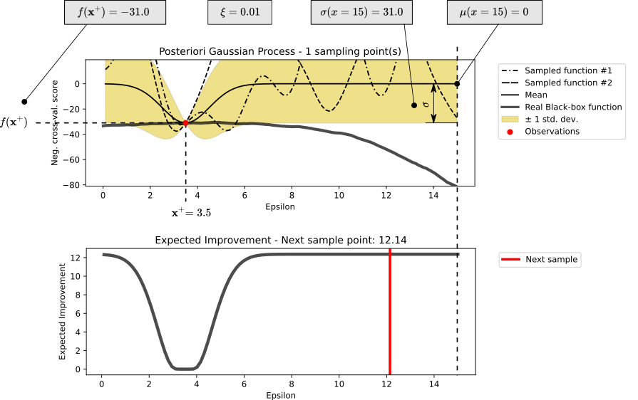
Each functional evaluation is costly, thus ruling out the option for an exhaustive probing. We need to have a sample-efficient method to minimize the number of evaluations of the environment while trying to locate its global optimum. In other words, the optimizer needs to fully utilize the existing observations and systematically reason about the next sampling decision so that the limited resource is not wasted on unpromising locations.
We do not have access to its gradient. When the functional evaluation is relatively cheap, and the functional form is smooth, it would be very convenient to compute the gradient and optimize using the gradient descent type of procedure. Without access to the gradient, we are unclear of the adjacent curvature of a particular evaluation point, thus making the follow-up direction of travel difficult.

Three possible functional forms. On the left is a convex function whose optimization is easy. In the middle is a nonconvex function with multiple local minina, and on the right is also a nonconvex function with a wide flat region full of saddle points. Optimization for the latter two cases is difficult. Image by the author.

The observation model

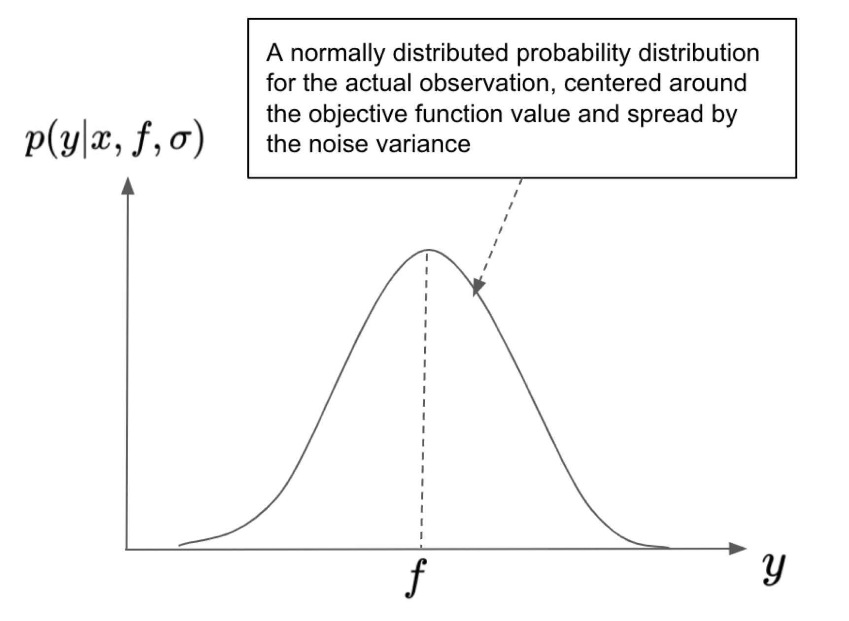
To make our discussion more precise, let us use f(x) to denote the (unknown) objective function value at location x. We use y to denote the actual observation at location x, which will slightly differ from f due to perturbation from an additive Gaussian noise. We can thus express the observation model as a probability distribution of y based on a specific location x and true function value f : p(y|x,f).

Assuming a normal probability distribution for the actual observation as a random variable. The Gaussian distribution is centered around the objective function f value evaluated at a given location x, and spread by the variance of the noise term. Image by the author.

Bayesian inference

Bayesian Inference essentially relies on the Bayesian formula (also called the Bayes’ rule) to reason about the interactions among a few components: the prior distribution, the likelihood given a specific parameter, and the posterior distribution, plus the evidence of the data.

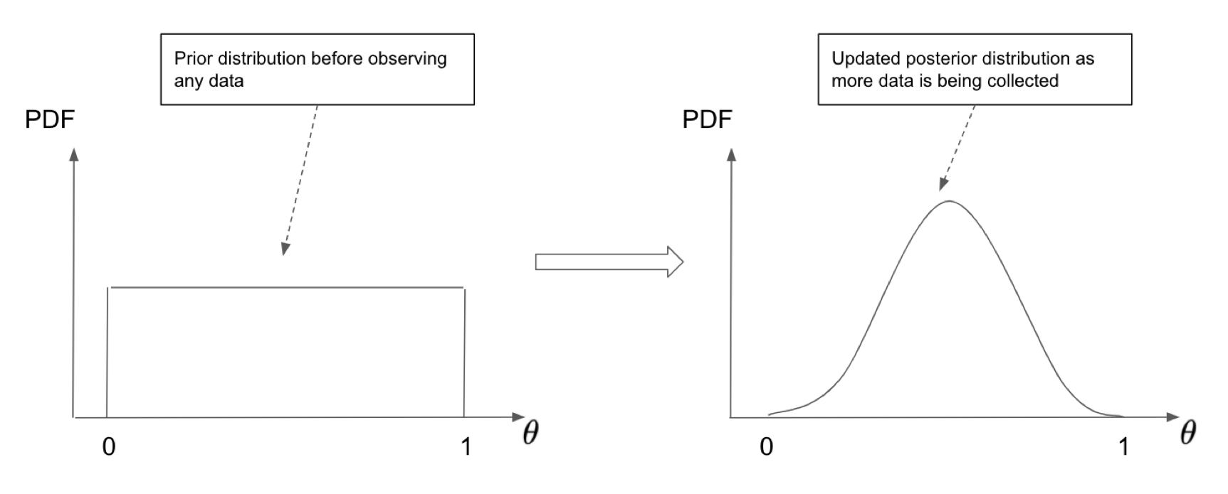
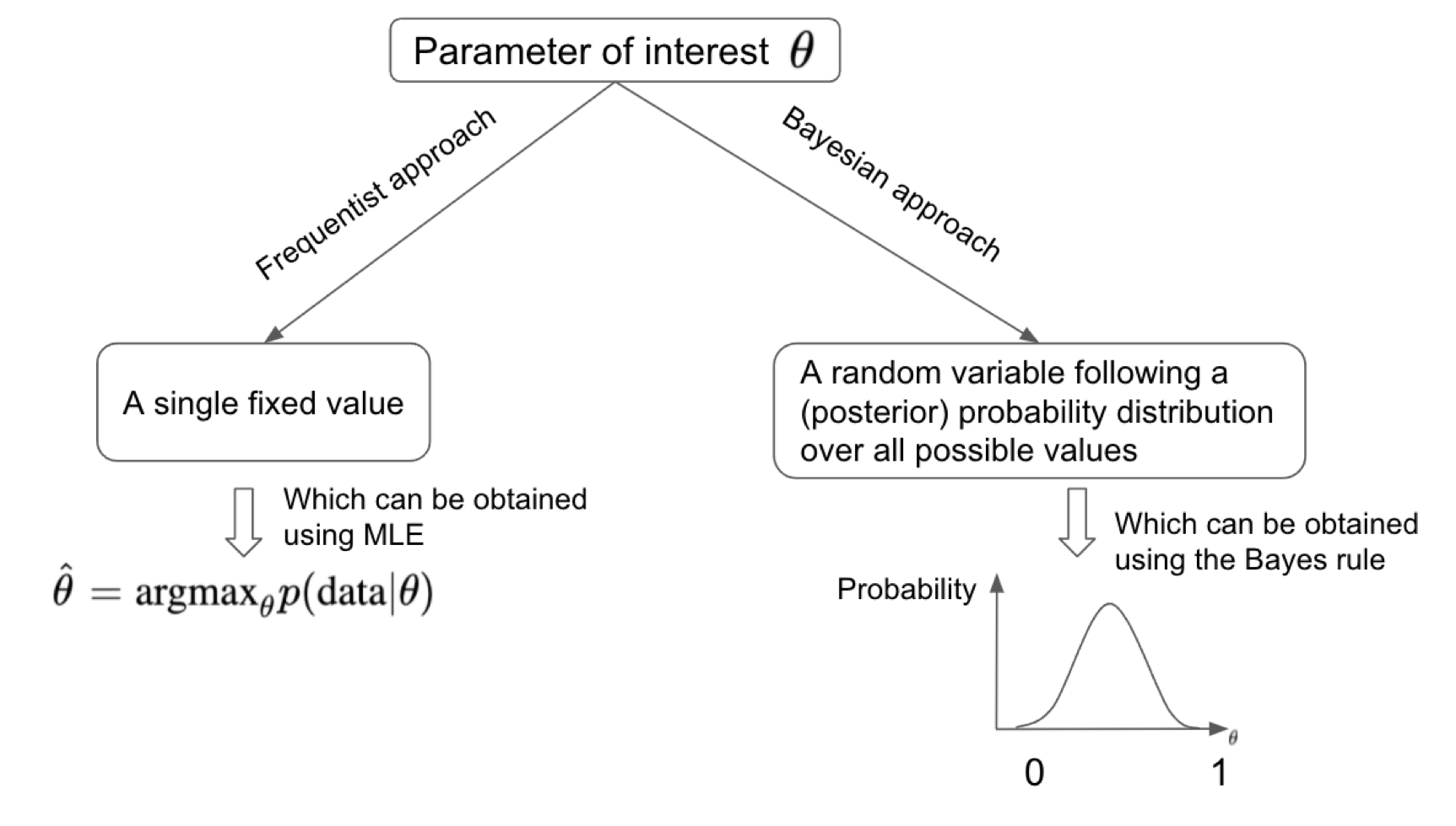
Updating the prior uniform distribution towards a posterior normal distribution as more data is being collected. The role of the prior distribution decreases as more data is collected to support the approximation to the true underlying distribution. Image by the author.

The Bayesian approach is a systematic way of assigning probabilities to possible values of parameters and updating these probabilities based on the observed data. However, sometimes we are only interested in the most probable value of parameters that gives rise to the data we are observing. This can be achieved using the frequentist approach, treating the parameter of interest as a fixed quantity instead of a random variable. This approach is more often adopted in the machine learning community that places a strong focus on optimizing a certain objective function to locate the optimal set of parameters.

Comparing the frequentist approach and the Bayesian approach regarding the parameter of interest. The frequentist approach treats the parameter as a fixed quantity that can be estimated via MLE, while the Bayesian approach employs a probability distribution that gets refreshed as more data is collected. Image by the author.

Things become more interesting when we work with multiple (more than one) variables. Suppose we have two random variables x and y, and we are interested in two _events x=_X and y=Y where both X and Y are specific values that x and y may assume respectively. Also, we assume the two random variables are dependent in some way. This would lead us to three types of probabilities that are commonly used in modern machine learning and Bayesian Optimization literature: joint probability, marginal probability, and conditional probability.

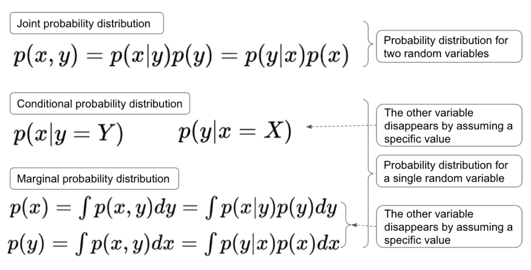
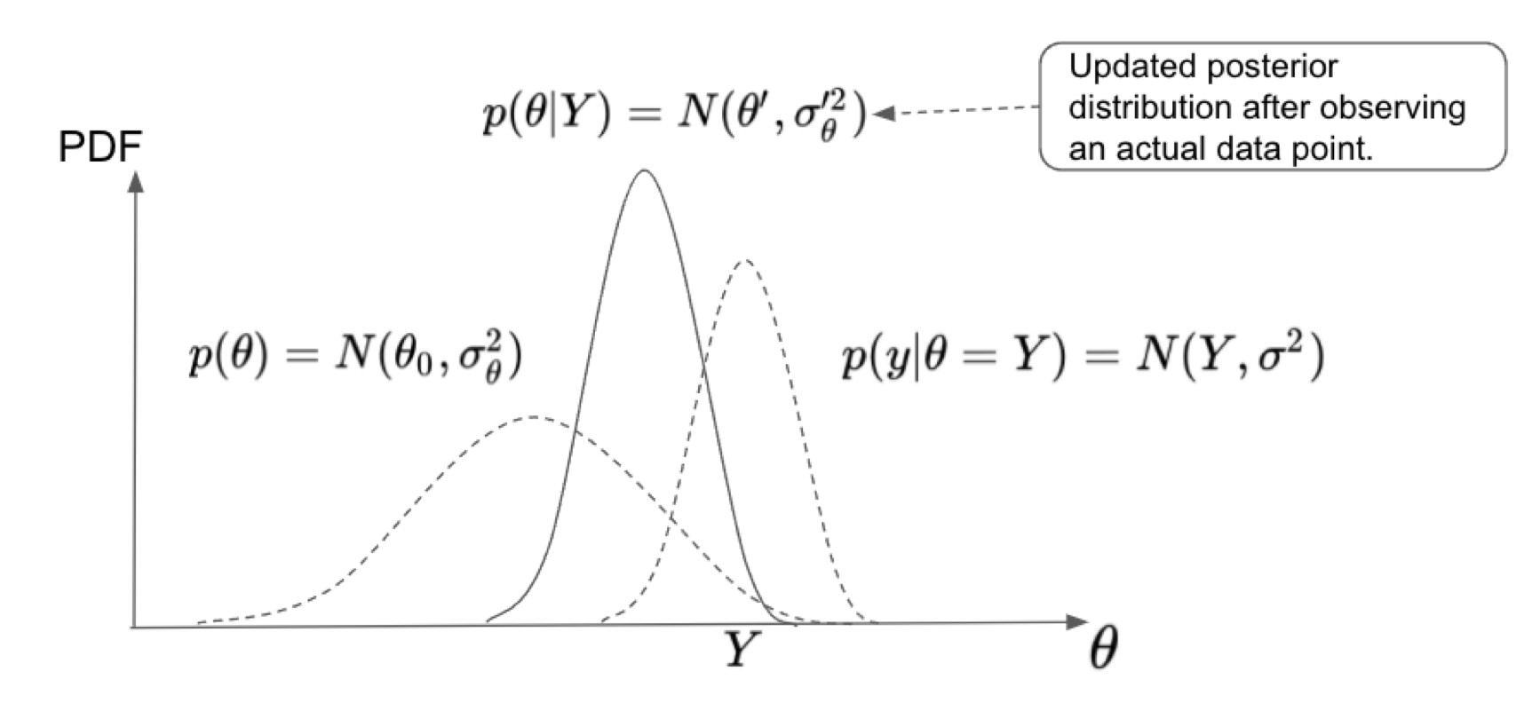
Three common probability distributions. The joint probability distribution represents the probability distribution for two or more random variables, while the conditional and marginal probability distributions generally refer to the probability distribution for one random variable. The conditional distribution represents the probabilities of a random variable by assuming/conditioning a specific value for other variables, while the marginal distribution converts a joint probability to a single random variable by integrating out other variables. Image by the author.

We are interested in its predictive distribution p(y), i.e., the possible values of y along with the corresponding probabilities. Our decision-making would be much more informed if we have a good understanding of the predictive distribution of the future unknown data, particularly in the Bayesian optimization framework where one needs to carefully decide the next sampling location.

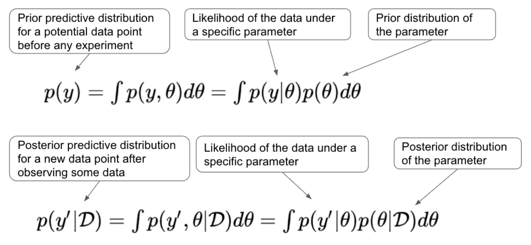
Definition of the prior and posterior predictive distributions. Both are calculated based on the same pattern of a weighted sum between the prior and the likelihood. Image by the author.

We can summarize the derivation of the posterior predictive distributions under the normality assumption for the likelihood and the prior for a continuous parameter of interest.

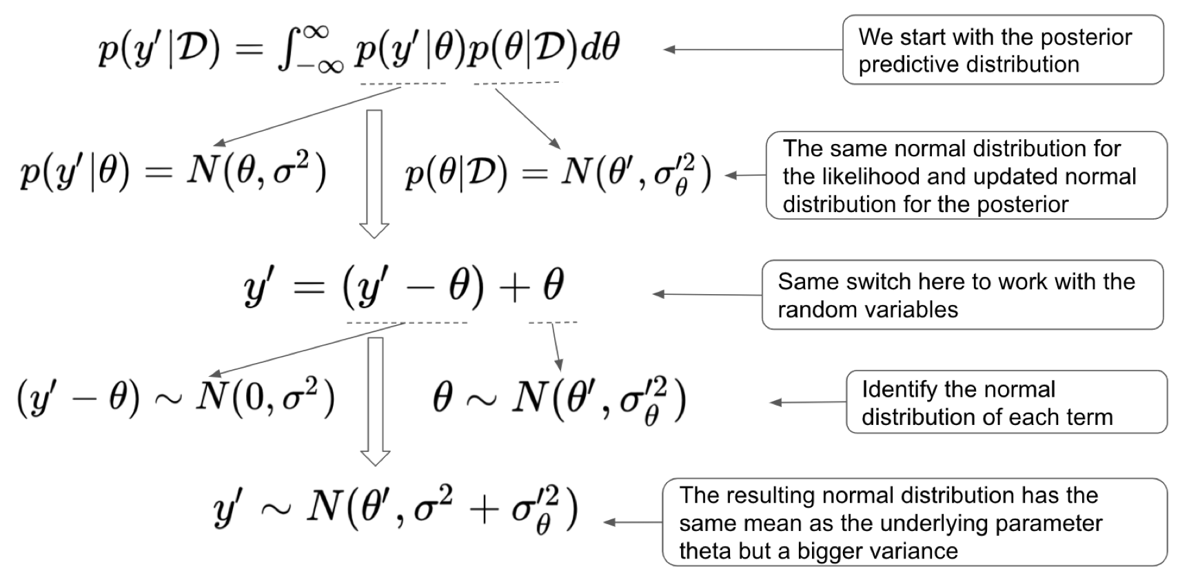
Derivation process of the posterior predictive distribution for a new data point after collecting some observations, assuming a normal distribution for both the likelihood and the prior. Image by the author.

With these tools available at hand, we can then the updated posterior distribution for the parameter of interest as well as the posterior predictive distribution for the random variable in a specific input location.

Updated the posterior distribution for the parameter, suggesting an alignment between subjective preference and reality. Image by the author.

Summary

This article covers some highlights of the Bayesian part in the framework of Bayesian optimization. In later articles, we will cover more essential contents such as the Gaussian process and acquisition function. For a more thorough and complete treatment on Bayesian optimization essential knowledge and implementation, please follow my Medium account and stay tuned for my upcoming book Practical Bayesian Optimization with Python.