Transfer Learning on Greyscale Images: How to Fine-Tune Pretrained Models on Black-and-White Datasets
Everything you need to know to understand why the number of channels matters and how to work around this
As the field of Deep Learning continues to mature, at this point it is widely accepted that transfer learning is the key to quickly achieving good results with computer vision, especially when dealing with small datasets. Whilst the difference that starting with a pretrained model will make partially depends on how similar the new dataset is to the original training data, it can be argued that it is almost always advantageous to start with a pretrained model.
Despite an ever-growing number of pretrained models available for image classification tasks, at the time of writing, the majority of these are trained on some version of the ImageNet dataset; which contains colour images. Whilst this is usually what we are looking for, in some domains - such as manufacturing and medical imaging - it is not uncommon to encounter datasets of black-and-white images.
As the difference between a colour image and a black-and-white image is trivial to us humans, you would be forgiven for thinking that a finetuning pretrained model should work out of the box, yet this is rarely the case. Therefore, especially if you have a limited background in image processing, it can be difficult to know what the best approach is to take in these situations,
In this article, we shall attempt to demystify all of the considerations needed when finetuning with black-and-white images by exploring the difference between RGB and greyscale images, and how these formats affect the processing operations done by convolutional neural network models, before demonstrating how to use greyscale images with pretrained models. We shall finish by examining the performance of the different approaches explored on some open source datasets and compare this to training from scratch on greyscale images.

What is the difference between RGB and grayscale images?
Whilst colour and greyscale images may very similar to us, as a computer only sees an image as an array of numbers, this can make a huge difference to how an image is interpreted! Therefore, to fully appreciate why greyscale images may pose a challenge for pretrained networks, we must first examine the differences in how colour and greyscale images are interpreted by a computer.
As an example, let’s use an image from the beans dataset.

RGB Images
Often, when we are working with colour images in deep learning, these are represented in RGB format. At a high level, RGB is an additive colour model where each colour is represented by a combination of red, green and blue values; these are usually stored as separate ‘channels’, such that an RGB image is often referred to as a 3 channel image.
We can check the mode — a string which defines the type and depth of a pixel in the image, as described here - of the image, as well as inspecting the available channels, using PIL as demonstrated below.
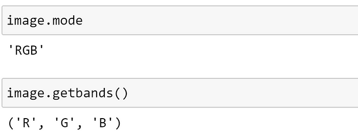
This confirms that PIL has recognised this as an RGB image. Therefore, for each pixel, the values stored in these channels — known as the intensities — each make up a component of the overall colour.
These components can be represented in different ways:
- Most commonly, the component values are stored as unsigned integer numbers in the range 0 to 255; the range that a single 8-bit byte can offer.
- In floating point representations, values can be represented from 0 to 1, with any fractional value in between.
- Each colour component value can also be written as a percentage, from 0% to 100%.
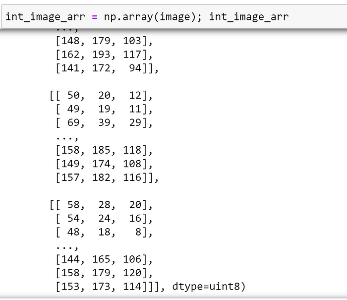
Converting our image to a NumPy array, we can see that, by default, the image is represented as an array of unsigned integers:
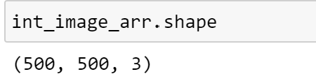
Inspecting the shape of the array, we can see that the image has 3 channels, which is in line with our expectations:
To convert our image array to a floating point representation, we can explicitly specify the dtype of the array at the time of creation. Let’s see what happens when we convert and plot our image.

Oh no!
From the warning message, which can be confirmed by inspecting the data, we can see that the reason the image is not displaying correctly because the input data is not in the correct range for floating point representation. To rectify this, let’s divide every element in the array by 255; which should ensure that each element is in the range [0, 1].

Plotting our normalised array, we can see that the image is now displaying correctly!
Understanding Component Intensities
By adjusting the intensity of each component, we can represent a wide range of colours using the RGB model.
When 0% intensity for each component is combined, no light is generated, so this creates black (the darkest possible colour).

When the intensities for all the components are the same, the result is a shade of grey, which is darker or lighter depending on the magnitude of the intensity.

When one of the components has an intensity which is stronger than the others, the resulting colour is closer to the primary colour with the strongest component (red-ish, green-ish, or blue-ish):

When 100% intensity for each component is combined, this creates white (the lightest possible colour).

Whilst this has hopefully provided an overview of RGB images, more detail about the RGB colour model can be found here.
Greyscale Images
Now that we have examined how we can represent colour images using the RGB colour model, let’s investigate how greyscale images differ from this.
A greyscale image is simply one in which the only colours represented are different shades of grey. Whilst we often refer to such images as “black and white” in everyday conversation, a truly “black and white image” would consist of only these two distinct colours, which is very rarely the case; making ‘greyscale’ the more accurate term.
As there is no colour information to represent for a greyscale image, less information needs to be stored for each pixel and an additive colour model is not required! For greyscale images, the only information we require is a single value to represent the intensity of each pixel; the higher this value, the lighter the shade of grey. As such, greyscale images usually consist of a single channel, where each pixel intensity is just a single number ranging from 0 to 255.
To explore this further, we can use PIL to convert our image to greyscale, as demonstrated below.

As before, we can inspect the mode and image channels using PIL.

From PIL’s documentation, we can see that L refers to a a single channel, greyscale image. Once again, we can confirm this by converting this image into an array and inspecting the shape.

Note that, as we only have only one channel, the channel dimension is dropped entirely by default; which can cause a problem for some deep learning frameworks. We can explicitly add the channel axis using NumPy’s expand_dims function.

In PyTorch, we can accomplish the same thing using the unsqueeze method, as demonstrated below:

Why does this affect pre-trained models?
After observing the differences between RGB and greyscale images, we may be starting to understand how these representations may pose a problem for a model; especially if the model has been pretrained on a dataset of images which are in a different format to the ones that we are currently training on.
At present, most of the pretrained models available have been trained on a version of the ImageNet dataset, which contains colour images in RGB format. Therefore, if we are finetuning on greyscale images, the input that we are providing to our pretrained model is substantially different to any input that it has previously encountered!
As, at the time of writing, convolutional neural networks (CNNs) are the most commonly used pretrained models for vision tasks, we shall restrict our focus to understanding how CNNs are affected by the number of channels in an image; other architectures are outside of the scope of this article! Here, we shall assume familiarity with CNNs, and how convolutions work - as there are excellent resources that cover these topics in detail - and focus on how this process will be affected by changing the number of input channels.
For our purposes, the key information to keep in mind is that the core building block of a CNN is a convolutional layer, which we can think of as a process which applies a set of filters (also known as kernels) — where a filter is just a small matrix, commonly 3x3 — as a sliding window across an image; performing an elementwise multiplication before summing the results. A great tool for understanding exactly how this works can be found here.
How does the number of channels affect filters?
In pre-deep learning computer vision, filters were created by hand for certain purposes, such as edge detection, blurring, etc. As an example, let’s consider a hand-crafted 3×3 filter for detecting horizontal lines:

Whilst the same filter ‘weights’ are used across the whole image during the sliding window operation, these weights are not shared across channels; meaning that a filter must always have the same number of channels as the input. Therefore, any filter that we would like to apply to a 3 channel RGB image, must also have 3 channels! The number of channels that a filter has is sometimes referred to as the ‘depth’.
Considering the horizontal line filter that we defined above, in order to apply this to a 3 channel image, we would need to increase the depth of this filter, such that it would be 3x3x3. As we would like the same behaviour for each channel, in this case, we can simply duplicate our 3x3 filter across the channel axis.
We can do this as demonstrated below:

Now that the depth of the filter is compatible with the number of channels, we are able to apply this filter to a 3 channel image!
To do this, for each channel, we multiply the elements of our sliding window portion of the image by the elements of the corresponding filter; which will result in a 3x3 matrix which represents the features corresponding to the current filter position for each channel. These matrices can then be summed to obtain the corresponding portion of our output feature map.
This process is illustrated below:

We can repeat this process, moving the position of the filter across the image, to obtain the complete output feature map. Note that, regardless of the number of channels of the input image, as the features for each channel are added together, the feature map will always have a depth of 1.
Convolutional Neural Networks
Now that we have explored how a manually defined filter can be applied to a 3 channel image, at this point, you may be wondering: where do CNNs come into this?
One of the key ideas behind CNNs is that, instead of having experts defining filters manually, these filters can be randomly initialised, and we trust the optimization process to ensure that these learn to detect meaningful features during training; visualisations of the types of filters learned by CNNs are explored here. Therefore, except for these filters being learned instead of defined, the overall process is largely the same!
Within a CNN, each convolutional layer contains the parameters corresponding to the filters that will be learned; the number of random filters initialised is a hyperparameter that we can specify. As we saw in the example above, each filter will result in a single channel feature map being created, so the number of filters initialised by the convolutional layer will determine the number of output channels.
As an example, suppose that we have a single channel image, and we would like to create a convolutional layer which learns a single 3x3 filter. We can specify this as demonstrated below:

Here, we expect that the dimensions of the filter should be the same as the single channel horizontal line filter that we defined earlier. Let’s confirm this by inspecting this layer’s ‘weight’ attribute:

Recalling that PyTorch stores the number of channels first by default, and noting that a batch dimension has been added for computational purposes, we can see that the layer has initialised a 3x3 filter, as we would expect!
Now, let’s create another convolutional layer, this time specifying that we have 3 input channels — to be able to handle an RGB image — and inspect the weights.

Similarly to when we extended our manually defined filter, the initialised filter now has the same depth as the number of input channels; which gives the dimensions of 3x3x3.
However, when we extended our manually defined filter, we simply duplicated the same weights. Here, the key difference is that the 3x3 weights for each channel will be different; enabling the network to detect different features for each channel. Therefore each kernel learns features based on, and specific to, each channel of the input image!
We can confirm this by inspecting the weights directly, as displayed below:

From this, we can see that the weights are different for the 3x3 filter that will be applied to each channel.
Whilst it is easy to adjust the initialised filter dimensions based on our input when creating a new convolutional layer, this becomes more difficult when we start to consider pre-trained architectures.
As an example, let’s examine the first convolutional layer of a Resnet-RS50 model, which has been pretrained on ImageNet, from the PyTorch Image models (timm) library; if you are unfamiliar with PyTorch Image models and would like to learn more, I have previously explored some of the features of this library here.

As this model was trained on RGB images, we can see that each filter is expecting a 3 channel input. Therefore, if we were to attempt to use this model on greyscale images with a single channel, this simply wouldn’t work as we are missing vital information; the filters would be trying to detect features in channels that don’t exist!
Additionally, in our previous examples we considered convolutional layers which would learn a single filter; which rarely the case in practice. Usually, we would like each convolutional layer to multiple filters, so that each of them will be able to specialize in identifying different features from the input. Depending on the task, some may learn to detect horizontal edges, others to detect vertical edges, etc. These features can be further combined by later layers, enabling the model to learn increasingly complex feature representations. Here, we can see that the convolutional layer from the ResNet-RS50 model has 32 output channels, meaning that it has learned 32 different filters, each requiring a 3 channel input!
How to use greyscale images with pretrained models
Now that we understand why greyscale images, with a reduced number of channels, are incompatible with pretrained models trained on RGB images, let’s explore some of the ways that we can overcome this!
In my experience, there tend to be two main approaches which are commonly used:
- Adding additional channels to each greyscale image
- Modifying the first convolutional layer of the pretrained network
Here, we shall explore both approaches.
Adding additional channels to greyscale images
Arguably, the simplest approach to use greyscale images with a pretrained model is to avoid modifying the model at all; instead, duplicating the existing channel so that each image has 3 channels. Using the same greyscale image that we saw earlier, let’s explore how we can do this.

Using NumPy
First, we need to convert our image into a NumPy array:

As we previously observed, because our image only has a single channel, the channel axis has not been created. Once again, we can use the expand_dims function to add this.

Now that we have created an additional axis for the channel dimension, all that we need to do is repeat our data over this axis; for which we can use the repeat method, as demonstrated below.

For convenience, let’s summarise these steps into a function, so that we can easily repeat this process if needed:
def expand_greyscale_image_channels(grey_pil_image):
    grey_image_arr = np.array(grey_image)
    grey_image_arr = np.expand_dims(grey_image_arr, -1)
    grey_image_arr_3_channel = grey_image_arr.repeat(3, axis=-1)
    return grey_image_arr_3_channel
Applying this function to our image, and plotting the output, we can see that the resulting image displays correctly, although now it has 3 channels.

Using PyTorch
If we are doing Deep Learning, it may be more useful to explore how we can do this conversion using PyTorch directly, rather than using NumPy as an intermediary. Whilst we could perform a similar set of steps as above on a PyTorch tensor, it is likely that we will want to perform additional transformations on our image — such as the data augmentation operations defined in TorchVision — as part of the training process. As we would like the 3-channel conversion to take place at the start of our augmentation pipeline, and some subsequent transforms may expect a PIL image, manipulating a tensor directly may not be the best approach here.
Thankfully, although somewhat counterintuitively, we can use the existing Grayscale transformation included in TorchVision to do this conversion for us! Whilst this transform expects either a torch tensor or a PIL image, as we would like this to be the first step in our pipeline, let’s use a PIL image here.
By default, this transform converts an RGB image to a single channel greyscale image, but we can modify this behaviour by using the num_output_channels argument, as demonstrated below.

Now, let’s see what happens if we apply this transform to our greyscale image.

At first glance, it doesn’t look although anything has changed. However, we can confirm the transform has worked as intended by inspecting the channels and mode of the PIL image.

As the additional channels have been added, we can see that PIL now refers to this image as an RGB image; which is what we wanted!
Therefore, the only modification required to a training script to use greyscale images, with this approach, would be to prepend this transform to the augmentation pipeline, as demonstrated below.

Modifying the first convolutional layer of the pretrained network
Whilst it can be convenient to expand a single channel image to 3 channels, as demonstrated above, a potential drawback of this is that additional resources are required to store and process the additional channels; which don’t provide any new information in this case!
A different approach is to modify the model to accommodate the different input which, in most cases, requires modifying the first convolutional layer. Whilst we could replace the whole layer with a new one, this would mean discarding some of the model’s learned weights and — unless we freeze the subsequent layers and train the new layer in isolation to begin with, which requires additional effort — the outputs coming from these new, randomly initialised weights may negatively disrupt some of the later layers.
Alternatively, recalling that each filter within a convolutional layer has separate channels, we can sum these together along the channel axis. Let’s explore how we can do this below. Once again, we shall use a Resnet-RS50 model from PyTorch Image models.
First, let’s create our pretrained model:

As we would expect, based on our earlier exploration of filters and channels, if we attempt to use this model on a single channel image out-of-the-box we observe the following error.

Let’s fix this by adjusting the weight of the first convolutional layer. For this model, we can access this as demonstrated below, but this will vary depending on the model used!

First, let’s update the in_channels attribute for this layer to reflect our change. This doesn't actually modify the weights, but will update the overview seen when printing the model as well as ensuring that we would be able to save and load the model correctly.

Now, let’s perform the actual weight update. We can do this using the sum method, ensuring that the keepdim argument is set to True to preserve the dimensions. The only 'gotcha' to watch out for is that, as a new tensor is created as a result of the sum operation, we have to wrap this new tensor in nn.Parameter; so that the new weights will be automatically added to the model's parameters.

Now, using this model with a single channel image, we can see that the correct shape has been returned!

Using timm
Whilst we could perform the above steps manually on any PyTorch model, timm already contains the functionality to do this for us! To modify a timm model in this way, we can use the in_chans argument when creating a model as demonstrated below.

Comparing performance on open source datasets
Now that we have investigated two ways that we can use greyscale images with pretrained models, you may be wondering which one to use; or whether it is better to simply train the model from scratch on the greyscale images!
However, due to the almost limitless combinations of models, optimizers, schedulers, and training policies that may be used, as well as differences in datasets, it is extremely difficult ascertain a general rule for this; it is likely that the ‘best’ approach may vary depending on the specific task that you are investigating!
Despite this, to gain a rough idea of how the approaches performed, I decided to train one of my favourite model-optimizer-scheduler combinations on three open-source datasets to see how the different approaches compared. Whilst it is likely that changing the training policy may affect how different approaches perform, for simplicity, the training process was kept relatively consistent; based on practices that I have found to work well.
Experiment Setup
For all experiment runs, the following were kept consistent:
- Model: ResNet-RS50
- Optimizer: AdamW
- LR scheduler: Cosine decay
- Data augmentation: Images were resized to 224, horizontal flip was used during training
- Initial LR: 0.001
- Max number of epochs: 60
All training was carried out using a single NVIDIA V100 GPU, with a batch size of 32. To handle the training loop, I used the PyTorch-accelerated library.
The datasets used were:
- Beans: Beans is a dataset of images of beans taken in the field using smartphone cameras. It consists of 3 classes, 2 disease classes and the healthy class.
- Rock papers scissors (RPS): Images of hands playing rock, paper, scissor game.
- Oxford Pets: A 37 category pet dataset with roughly 200 images for each class.
For each dataset, I explored the following approaches to handling greyscale images:
- RGB: finetune the model using RGB images to act as a baseline.
- Greyscale w/ 3 channels: the greyscale images were converted to 3 channel format.
- Greyscale w/ 1 channel: the first layer of the model was converted to accept a single channel image.
Where relevant for each approach, I used the following training policies:
- Finetune: using a pretrained model, first train the model’s final layer, before unfreezing and training the whole model. After unfreezing, the learning rate is reduced by a factor of 10.
- Finetune whole model: train the entire pretrained model, without freezing any layers.
- From scratch: train the model from scratch
The training script used to run this experiment is provided below, the package versions used were:
- PyTorch: 1.10.0
- PyTorch-accelerated: 0.1.22
- timm: 0.5.4
- torchmetrics: 0.7.1
- pandas: 1.4.1
Results
The results of these runs are presented in the table below.

From these experiments, my main observations are:
- It appears to be easier to achieve good results using a pretrained model, and adapting this to use greyscale images, rather than training from scratch.
- The best approach on these datasets appears to be modifying the number of channels in the image rather than modifying the model.
Conclusion
Hopefully, this has provided a reasonably comprehensive overview of how to finetune pretrained models on greyscale images, as well as an understanding of why additional considerations are required.
Chris Hughes is on LinkedIn.
References
- ImageNet (image-net.org)
- RGB color model — Wikipedia
- Concepts — Pillow (PIL Fork) 9.1.0.dev0 documentation
- fastbook/13_convolutions.ipynb at master · fastai/fastbook (github.com)
- deeplizard — Convolution Demo
- LNCS 8689 — Visualizing and Understanding Convolutional Networks (nyu.edu)
- Revisiting ResNets: Improved Training and Scaling Strategies (arxiv.org)
- rwightman/pytorch-image-models: PyTorch image models, scripts, pretrained weights — ResNet, ResNeXT, EfficientNet, EfficientNetV2, NFNet, Vision Transformer, MixNet, MobileNet-V3/V2, RegNet, DPN, CSPNet, and more (github.com)
- Getting Started with PyTorch Image Models (timm): A Practitioner’s Guide | by Chris Hughes | Feb, 2022 | Towards Data Science
- Chris-hughes10/pytorch-accelerated: A lightweight library designed to accelerate the process of training PyTorch models by providing a minimal, but extensible training loop which is flexible enough to handle the majority of use cases, and capable of utilizing different hardware options with no code changes required. Docs: https://pytorch-accelerated.readthedocs.io/en/latest/ (github.com)
Datasets Used
- Beans Dataset, AI-Lab-Makerere/ibean: Data repo for the ibean project of the AIR lab. (github.com). MIT License, use without restriction.
- Rock, Paper, Scissors Dataset, Laurence Moroney Datasets for Machine Learning — Laurence Moroney — The AI Guy. CC By 2.0 license, free to share and adapt for all uses, commercial or non-commercial
- Oxford Pets Dataset, Visual Geometry Group — University of Oxford. Creative Commons Attribution-ShareAlike 4.0 International License, including commercial and research purposes.

