Training Deep Neural Networks
Deep Learning Accessories
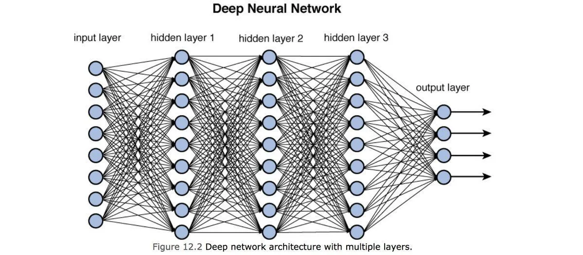
Deep neural networks are key break through in the field of computer vision and speech recognition. For the past decade, deep networks have enabled the machines to recognize images, speech and even play games at accuracy nigh impossible for humans. To achieve high level of accuracy, huge amount of data and henceforth computing power is needed to train these networks. However, despite the computational complexity involved, we can follow certain guidelines to reduce the time for training and improve model accuracy. In this article we will look through few of these techniques.
Data Pre processing
The importance of data pre-processing can only be emphasized by the fact that your neural network is only as good as the input data used to train it. If important data inputs are missing, neural network may not be able to achieve desired level of accuracy. On the other side, if data is not processed beforehand, it could effect the accuracy as well as performance of the network down the lane.
Mean subtraction (Zero centering)
It’s the process of subtracting mean from each of the data point to make it zero-centered. Consider a case where inputs to neuron (unit) are all positive or all negative. In that case the gradient calculated during back propagation will either be positive or negative (same as sign of inputs). And hence parameter updates are only restricted to specific directions which in turn will make it inefficient to converge.

Data Normalization
Normalization refers to normalizing the data to make it of same scale across all dimensions. Common way to do that is to divide the data across each dimension by it’s standard deviation. However, it only makes sense if you have a reason to believe that different input features have different scales but they have equal importance to the learning algorithm.

Parameter Initialization
Deep neural networks are no stranger to millions or billions of parameters. The way these parameters are initialized can determine how fast our learning algorithm would converge and how accurate it might end up. The straightforward way is to initialize them all to zero. However, if we initialize weights of a layer to all zero, the gradients calculated will be same for each unit in the layer and hence update to weights would be same for all units. Consequently that layer is as good as a single logistic regression unit.
Surely, we can do better by initializing the weights with some small random numbers. Isn’t it? Well, let’s analyse the fruitfulness of that hypothesis with a 10 layer deep neural network each consisting of 500 units and using tanh activation function. [Just a note on tanh activation before proceeding further].

On the left is the plot for tanh activation function. There are few important points to remember about this activation as we move along :-
- This activation is zero-centered.
- It saturates in case input is large positive number or large negative number.
To start with, we initialize all weights from a standard Gaussian with zero mean and 1 e-2 standard deviation.
W = 0.01 * np.random.randn(fan_in, fan_out)Unfortunately, this works well only for small networks. And to see what issues it creates for deeper networks plots are generated with various parameters. These plots depict the mean, standard deviation and activation for each layer as we go deeper into the network.


Notice that mean is always around zero, which is obvious since we are using zero centered non-linearity. However, standard deviation is shrinking gradually as we go deeper into the network till it collapses to zero. This, as well, is obvious on account of the fact that we are multiplying the inputs with very small weights at each layer. Consequently, the gradients calculated would also be very small and hence update to weights will be negligible.
Well not so good!!! Next let’s try initializing weights with very large numbers. To do so, let’s sample weights from standard Gaussian with zero mean and standard deviation as 1.0 (instead of 0.01).
W = 1.0 * np.random.randn(fan_in, fan_out)Below are the plots showing mean, standard deviation and activation for all layers.


Notice, the activation at each layer is either close to 1 or -1 since we are multiplying the inputs with very large weights and then feeding it to tanh non-linearity (squashes to range +1 to -1). Consequently, the gradients calculated would also be very close to zero as tanh saturates in these regimes (derivative is zero). Finally, the updates to weight would almost again be negligible.
In practice, Xavier initialization is used for initializing the weights of all layers. The motivation behind Xavier initialization is to initialize the weights in such a way they do not end up in saturated regimes of tanh activation i.e initialize with values not too small or too large. To achieve that we scale by the number of inputs while randomly sampling from standard Gaussian.
W = 1.0 * np.random.randn(fan_in, fan_out) / np.sqrt(fan_in)However, this works well with the assumption that tanh is used for activation. This would surely break in case of other activation functions for e.g — ReLu. No doubt that proper initialization is still an active area of research.
Batch normalization
This is somewhat related idea to what all we discussed till now. Remember, we normalized the input before feeding it to our network. One reason why this was done was to take into account the instability caused in the network by co-variance shift.
It explains why even after learning the mapping from some input to output, we need to re-train the learning algorithm to learn the mapping from that same input to output in case data distribution of input changes.
However, the issue isn’t resolved there only as data distribution could vary in deeper layers as well. Activation at each layer could result in different data distribution. Hence, to increase the stability of deep neural networks we need to normalize the data fed at each layer by subtracting the mean and dividing by the standard deviation. There’s an article that explains this in depth.
Regularization
One of the most common problem in training deep neural network is over-fitting. You’ll realize over-fitting in play when your network performed exceptionally well on the training data but poorly on test data. This happens as our learning algorithm tries to fit every data point in the input even if they represent some randomly sampled noise as demonstrated in figure below.

Regularization helps avoid over-fitting by penalizing the weights of the network. To explain it further, consider a loss function defined for classification task over neural network as below :

J(theta) - Overall objective function to minimize.
n        - Number of training samples.
y(i)     - Actual label for ith training sample.
y_hat(i) - Predicted label for ith training sample.
Loss     - Cross entropy loss.
Theta    - Weights of neural network.
Lambda   - Regularization parameter.
Notice how, regularization parameter (lambda) is used to control the effect of weights on final objective function. So, in case lambda takes a very large value, weights of the network should be close to zero so as to minimize the objective function. But as we let weights collapse to zero, we would nullify the effect of many units in the layer and hence network is no better than a single linear classifier with few logistic regression units. And unexpectedly, this will throw us in the regime known as under-fitting which is not much better than over-fitting. Clearly, we have to choose the value of lambda very carefully so that at the end our model falls into balanced category(3rd plot in the figure).
Dropout Regularization
In addition to what we discussed, there’s one more powerful technique to reduce over-fitting in deep neural networks known as dropout regularization.
The key idea is to randomly drop units while training the network so that we are working with smaller neural network at each iteration. To drop a unit is same as to ignore those units during forward propagation or backward propagation. In a sense this prevents the network from adapting to some specific set of features.

At each iteration we are randomly dropping some units from the network. And consequently, we are forcing each unit to not rely (not give high weights) on any specific set of units from previous layer as any of them could go off randomly. This way of spreading the weights eventually shrinks the weights at individual unit level similar to what we discussed in L 2 regularization.
Much of the content can be attributed to
Please let me know through your comments any modification/improvements needed in the article.