Time Series Land Cover Challenge: a Deep Learning Perspective
A quick review of different DL architectures for the TiSeLaC challenge
Presented back in 2017 by the Université de Montpellier, the TiSeLaC challenge [1] (TiSeLaC for Time Series Land Cover) consists in predicting Land Cover class of pixels in Time Series of satellite images.

Table of Contents
- What is Time Series Satellite Imagery
- What about TiSeLaC dataset ?
- TiSeLaC classification task
- Conclusion
1. What is Time Series Satellite Imagery?
Time Series Satellite Imagery is the addition of a temporal dimension to Satellite Imagery. In other words, it is a series of satellite pictures taken at a regular interval in order to use not only the spatial information embedded in the picture but also the temporal dimension to make a prediction, whether these predictions are classification, detection or segmentation.
One of the most historically noticeable uses of time series of satellite imagery was back in 2002 by X. Yang & C. P. Lo [2] where they revealed and quantified loss of forest as well as urban sprawl in the context of Atlanta’s accelerated urban development.
2. What about TiSeLaC dataset?
These satellites pictures are 23 images of 2866 * 2633 pixels of La Réunion Island taken in 2014 at a 30m resolution. Each of these pixels is made up of 10 features: 7 surface reflectances representing measures of each independent multi-spectral band (OLI): Ultra Blue, Blue, Green, Red, NIR, SWIR1 and SWIR2. We find as well 3 complementary radiometric indices with the Normalized Difference Vegetation Index, the Normalized Difference Water Index as well as, finally, the Brightness index.
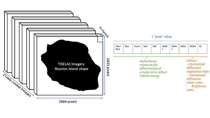
With that many bands, we can only imagine potential correlation between bands. We will now dive deeper into Exploratory Data Analysis.
2.1 Exploratory Data Analysis
First important thing to note here is that out of the 2866*2633 pixels contained in every image, only 81714 were retained in the training set, as well as 17973 pixels for the test set. This means that we do NOT work with entire images, as only subsets of pixels are processed and analysed.
The following animation displays the Blue, Green and Red components of each pixels with variations in time:

Also, to have an overview of every class raster, I have created a plot for each class by computing the respective mean and standard deviation of the ten bands for each of the 23 total days.
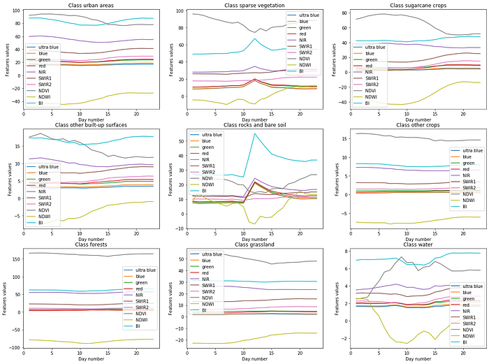
As we can see there, a few different classes see their features be highly disturbed through the days (e.g the water class or the rocks and bare soil are the most noticeable). Oppositely, the forests and crops classes are pretty steady in their results.
This apparent diversity in the variation of the features for each class is a “good sign”, it should not be too hard for an automatic classifier to be able to discriminate them from each other. However, these results are generalizing at best and can be misleading, they just provide insights on data diversity but are not proofs that the task of classification, or at least highly accurate classification, will be easy.
We will now explore the classes distributions. The subsampling of the pixels done by the TiSeLaC organizers had, as a first intent, the idea of balancing the classes distribution. We are then expecting to see a somewhat balanced dataset:

We see that the dataset is actually skewed with the “other crops” class having lass than 2000 training examples while the urban areas, the forests and the sparse vegetation all are upsampled.
For the test set, we have:

We have here a somewhat similar plot with every class being between 4 to 6 times less present than in the training set except for the “other crops” that are even rarer on the test set.
2.2 First hints for the classification problem
As this dataset is made of subsampled data, in a way that only some of the pixels are retained, we cannot attack the problem as image processing as we only have access to parts of the image.
However, we can see the problem from the point of view of signal processing, and more especially of Time Series classification with extra information concerning the localisation of the said time series in space thanks to pixels coordinates data.
3. TiSeLaC Classification task
Once we take the direction of Time Series classification, we can compare different models that have been popular in recent Deep Learning for Time Series litterature.
3.1 Multiple unimodal networks: Multi-Channel Deep Convolutional Neural Network
One of the most popular models being the Multi-Channel Deep Convolutional Neural Network (i.e. MCDCNN) developed and studied in [3]. This architecture want to exploit a presumed independence between the different features of the mutlimodal time series data by applying convolution independently (i.e. in parallel) on each dimension of the input.
I implemented one myself for this task using Python and Keras.
First, I describe the individual architecture for each of the 10 channels:
Then I mixed them into a single model with a Concatenate layer.
For the training procedure, I used a SGD with a learning rate of 0.01, a decay of 0.0005, a batch size of 64 instances as well as 120 epochs.
Considering the F1 score metric used by the TiSeLaC organizers as a marking scheme, I reached the score of 0.867
However, an assessment that is to be made for this dataset is that we are dealing with multimodal time series.
3.2 Multimodal network: Time-CNN
Indeed, one may argue that the value of indices are correlated with the values of the reflectance measures. This is especially noticeable with the plot of the “rocks and bare soil” class where a peak in mutiple band is noticeable around day 11.
This idea has been treated in [4] by Zhao B, Lu H, Chen S, Liu J and Wu D where they introduced the concept of the Time-CNN. This model differs from the MCDCNN in multiple ways:
- it uses a MSE loss with a sigmoid output layer, instead of the usual categorical crossentropy and of the softmax output layer;
- it uses Average Pooling instead of the usual Max Pooling;
- No pooling layer is present after the last Convolutional layer
My implementation of the Time-CNN, once again in Keras and Python, is the following:
This time, I used a learning rate of 1e-3, the Adam optimizer with no decay, a batch size of 128 and 100 epochs (with EarlyStopping that usually stops the training processaround 50 epochs).
With this technique, I achieved a F1 score of 0.878 which is correct but still not satisfying.
As we have seen, both models take radically different angle when thinking about how to work on this task: one make the supposition that the time series are uncorrelated while the other consider the 10 time series as being a unique entity. This is where I thought that using both ideas and merging them into a single model would help.
3.3 Combination of multimodal and multiple unimodal architectures
This idea was intensively explored in [5] by a team of researchers of the TiSeLaC competition that reached the top position with their solution. My implementation is highly inspired by their work and although I did not reach the same performance as they did (the reasons being that they used preprocessed spatial feature representation of pixels as well as the usual Time Series, completed with bagging techniques of multiple models initialized differently), I still managed to get a satisfying score.
My architecture was the following:

The proposed architecture uses 3 different models, starting with a multivariate model on the left, 10 univariate models at the middle and an aggregating model for position information on the right.
The first model, the univariate, only comprises of 3 convolutional layers with no pooling layers in between.
The second model uses 10 univariate models with different level of concatenation to work with features engineered at different levels of the network, somewhat similar to what a UNet or a ResNet would do.
Then, the third model just passes through the preprocessed and scaled pixel coordinates to the final fully-connected layers.
Then, each of these feature extraction models outputs are concatenated to be classified with usual fully-connected layers:
With this architecture, I obtained a F1 score of 0.930 with a learning rate of 0.001, a batch size of 256, 50 epochs and an Adam optimizer with default parameters.

With this score, my solution would be positioned right above the GIT team. However, it still needs thorough hyperparameter tuning by running possible GridSearch algorithms on a highly performant computer as well as finding a good preprocessing idea for the pixel positions, instead of a simple scaling procedure.
4. Conclusion
We have seen through this project how efficient nowadays DL architecture are to classify Time Series data and how merging unimodal and multimodal analysis leads to better performance.
As a more general conclusion, we have seen how good Deep Learning is at working with sequences.
For a last note, I wanted to thank the organizer of the TiSeLaC competition for having made the dataset public. This way, I have been able to work through it and to learn more about building efficient models that do not require millions of parameters.
The whole code and execution procedure is stored in a Jupyter Notebook hosted on my personal GitHub at this link. Go check it out !
Bibliography
[1] R. Gaetano, D. Ienco. TiSeLaC : Time Series Land Cover Classification Challenge Dataset. UMR TETIS, Montpellier, France. 2017
[2] X. Yang, C. P. Lo. Using a time series of satellite imagery to detect land use and land cover changes in the Atlanta, Georgia metropolitan area. International Journal of Remote Sensing. p. 1775–1798. 2002.
[3] Y. Zheng, Q. Liu, E. Chen, Y. Ge, J. L. Zhao. Exploiting Multi-Channels Deep Convolutional Neural Networks for Multivariate Time Series Classification. Frontiers of Computer Science. 2014.
[4] Zhao B, Lu H, Chen S, Liu J, Wu D. Convolutional neural networks for time series classification. Journal of Systems Engineering and Electronics. p.162–169. February 2017.
[5] N. Di Mauro, A. Vergari, T. M. A. Basile, F. G. Ventola, F. Esporito. End-to-end Learning of Deep Spatio-temporal Representations for Satellite Image Time Series Classification. 2017.


