The Ultimate Beginner’s Guide To Implement A Neural Network From Scratch
Learning the calculus and mathematics behind neural networks and converting equations to code.
Abstract
Neural networks have been with us for a long time but they have gathered importance in recent years due to advancement in computing machinery as well as growing needs of technology in various aspects of life.
From the perspective of a beginner in machine learning, a neural network is considered as a black box which can ingest some data and spit out predictions or classification categories depending upon the problem at hand. The beauty of neural networks is that they are based on simple calculus and linear algebra or a combination of both. These work together to come up with close to accurate results when provided with high quantity and quality data.
So, if you are motivated to learn the basics of how a neural network actually works, you have reached the right place. Follow me along this post and you’ll be able to build your own neural network from scratch.
What Are Neural Networks?
A neural network’s architecture is derived from the structure of a human brain while from a mathematical point of view, it can be understood as a function which maps a set of inputs to desired outputs. The main idea of this post is to understand this function in detail and implementing it in python.
A neural network comprises of 7 Parts :
- Input Layer (X) : This layer contains the values corresponding to the features in our dataset.
- A set of weights and biases (W₁,W₂,..etc); (b₁,b₂,..etc) : These weights and biases are represented in the form matrices and they decide the importance of each feature/column in our dataset.
- Hidden Layer : This layer acts as a brain of the neural network and also as an interface between the input and the output layer. There can be one or more than one hidden layers in a neural network.
- Output Layer (ŷ) : The values transmitted from the input layer will reach this layer via the hidden layer(s).
- A set of activation functions (A) : This is the component which adds a non-linearity flavour to an otherwise linear model. These functions are applied to the output of each layer except the input layer and activate/transform them.
- The Loss function (L) : This function calculates the measure as to how well our guess/prediction is, and it is used while back propagating through the network.
- Optimiser : This optimiser is a function that updates the model parameters according to gradients which are calculated during back propagation (You’ll learn shortly).
The Learning Process
Neural networks learn/train from the training data and then their performance is tested using test data. There are 2 parts of the training process:
- Feed forward
- Back-propagation
Feed forward is basically traversing the neural network from input layer to the output layer by predicting a value. On the other hand, back-propagation makes the network actually learn by computing gradients and pushing them back through the network and finally updating the model parameters. Let us first see how these 2 processes work on paper and then we will convert our equations into code.
Let us first design our neural network architecture. The architecture which we will be using for this post is shown below:
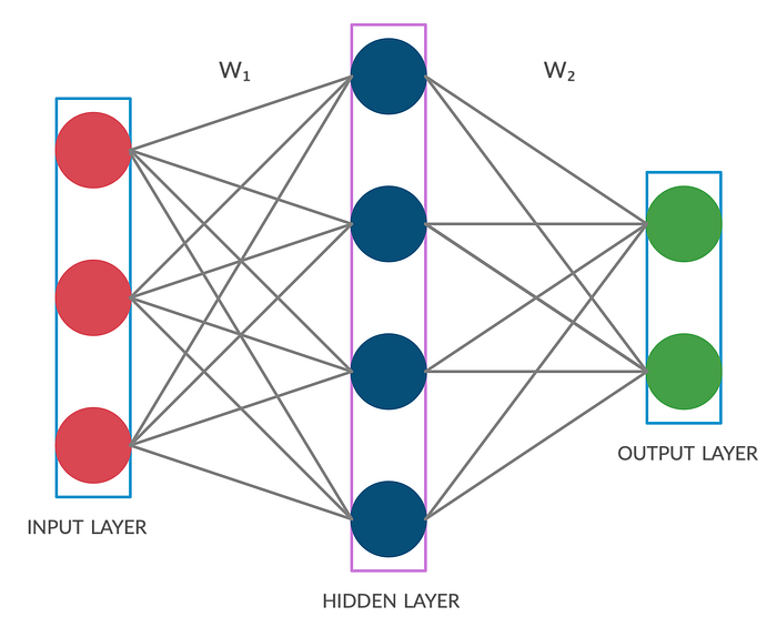
Feed Forward
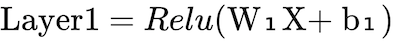
As far as our architecture is concerned, we just need 2 equations to carry out the feed forward process and for future purposes, you may remember:
number of layers of the neural network = number of hidden layers + 1(output layer)
number of weight matrices = number of layers
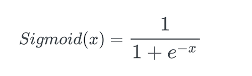
We will be using ReLu and Sigmoid activation functions in this post but other activation functions can alse be applied.

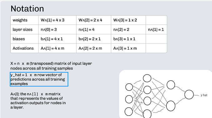
Here, X, W₁, b₁, W₂ and b₂ are matrices and matrix level computations are done in both the equations above. For better understanding, we can have a look at these matrices representing X, W₁, b₁, W₂ and b₂. In this post, we are ignoring the bias terms b₁ and b₂ but they can be dealt with in a similar manner.
Let us define a few values first :
n₁= number of neurons in the input layer, n₂= number of neurons in the hidden layer, n₃= number of neurons in the output layer.
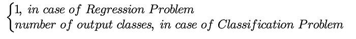
Now, you might be thinking of how to decide the number of neurons for Input layer, hidden layer and output layer. Here is the answer.
number of neurons in the input layer (n₁)= number of features/columns in our dataset i.e. the number of independent variables.
number of neurons in the hidden layer (n₂) is flexible.
number of neurons in the output layer (n₃) =

Dimensions of X: [m, n₁] ; Dimensions of W₁: [n₁, n₂] ;
Dimensions of W₂: [n₂, n₃]
Back Propagation
Back propagation is an essential part in training a neural network. It is a method of learning on the basis of gradients which are calculated using the most beautiful part of calculus i.e. the Chain Rule. This chain rule is repetitively applied to calculate gradients across the network. To make it more clear, a gradient is the derivative of loss function w.r.t. to a model parameter (weight or bias).
As mentioned earlier, we won’t be using bias terms and will only consider weights as model parameters. So, we have 2 model parameters i.e. W₁ and W₂. The loss function which we will be using is MSE (Mean Square Error). Now let us see how back propagation actually works mathematically.

where m= number of training examples/rows in the dataset
y= ground truth/label in the dataset
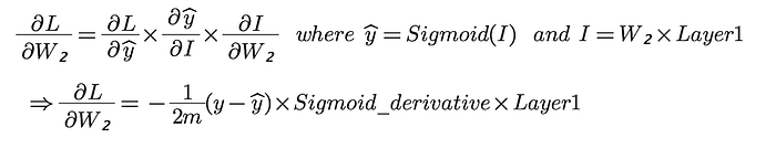
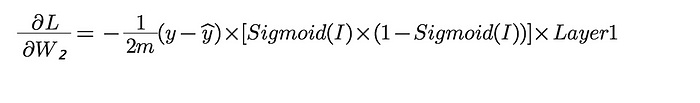
Let us calculate the gradient of loss w.r.t. W₂ using chain rule :
The derivation of ‘Sigmoid_derivative’ term is not in context of this post but it has been beautifully explained here.
Therefore, our first gradient term simply turns out to be :
Now, moving further, we calculate our second gradient term i.e. the derivative of loss w.r.t. W₁ in a similar way :

You can also refer to this post to know more about these activation functions and their derivatives.
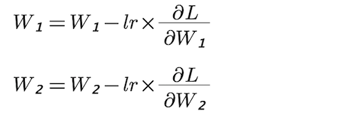
So, now that we have calculated the gradients w.r.t. W₁ and W₂, it is time to perform the optimisation steps. We will be using Gradient Descent Optimizer which is also called Vanilla Gradient Descent to update W₁ and W₂. You might be knowing that gradient descent algorithm has a hyper-parameter named as learning rate, which has a great importance in the training process. Tuning of this hyper-parameter is very essential and is done by using validation testing which is not in scope of this post.
Now that we have learnt the mathematical concepts behind a neural network, let us convert these concepts into code and train a neural network on a real-world machine learning problem. We will be using the famous IRIS dataset to train our network and then predict flower categories. You can download the dataset from here.
Implementing A Neural Network in Python
Importing Necessary Libraries
import numpy as np
import pandas as pd
from sklearn import preprocessing
from sklearn.preprocessing import StandardScaler
from sklearn.preprocessing import LabelEncoder
from sklearn.model_selection import train_test_split
Data Loading and Preprocessing
data=pd.read_csv('IRIS.csv')
X=data.iloc[:,:-1].values
Y=data.iloc[:,-1].values
StandardScaler=StandardScaler()
X=StandardScaler.fit_transform(X)
label_encoder=LabelEncoder()
Y=label_encoder.fit_transform(Y)
Y=Y.reshape(-1,1)
enc=preprocessing.OneHotEncoder()
enc.fit(Y)
onehotlabels=enc.transform(Y).toarray()
Y=onehotlabels
After doing aforesaid basic pre-processing on the input data, we move on to create our neural network class which contains the feed forward and back-propagation functions. But first, let us split our data into train and test.
X_train,X_test,Y_train,Y_test=train_test_split(X,Y,test_size=0.2,random_state=0)I am also writing code to define functions which can calculate function values and function derivative values. I have written code for 3 activation functions and used only two (Relu and Sigmoid) out of them. However, you can try out various combinations of these activation functions and also incorporate other activation functions in your code.
def ReLU(x):
   return (abs(x.astype(float))+x.astype(float))/2def ReLU_derivative(x):
   y=x
   np.piecewise(y,[ReLU(y)==0,ReLU(y)==y],[0,1])
   return ydef tanh(x):
   return np.tanh(x.astype(float))def tanh_derivative(x):
   return 1-np.square(tanh(x))def sigmoid(x):
   return 1/(1+np.exp(-x.astype(float)))def sigmoid_derivative(x):
   return x*(1-x)
Defining the neural network class :
class Neural_Network:
   def __init__(self,x,y,h):
      self.input=x
      self.weights1=np.random.randn(self.input.shape[1],h)
      self.weights2=np.random.randn(h,3)
      self.y=y
      self.output=np.zeros(y.shape)
The class ‘Neural_Network’ accepts 3 parameters: x, y and h which are corresponding to X_train, Y_train and number of neurons in the hidden layer. As mentioned earlier, number of neurons in the hidden layer is flexible and therefore we will pass its value along with X_train and Y_train while creating an instance of our class.
‘weights1’ and ‘weights2’ matrices are initialized from a random distribution and by passing the dimensions required for the respective weight matrices. As previously W₁ and W₂ matrices have been shown along with their dimensions, we pass these dimensions to this random function to generate our initial weights.
   def FeedForward(self):
      self.layer1=ReLU(np.dot(self.input,self.weights1))
      self.output=sigmoid(np.dot(self.layer1,self.weights2))
Our first function in the class is ‘FeedForward’ which is the first step in the training process of a neural network. The code follows ‘Equation-1’ and ‘Equation-2’ described earlier.
Next, we move on to the most essential part, the back-propagation.
def BackPropogation(self):
      m=len(self.input)
      d_weights2=-(1/m)*np.dot(self.layer1.T,(self.y-self.output)       *sigmoid_derivative(self.output))d_weights1=-(1/m)*np.dot(self.input.T,(np.dot((self.y-    self.output)*sigmoid_derivative(self.output),self.weights2.T)*    ReLU_derivative(self.layer1)))self.weights2=self.weights2 - lr*d_weights2
      self.weights1=self.weights1 - lr*d_weights1
The back-propagation step calculates gradients w.r.t. the model parameters while traversing back in the network from output layer to the input layer. This is governed by ‘Equation-3’ and ‘Equation-4’ which we obtained using chain rule. You will observe that both the terms ‘d_weights2’ and ‘d_weights1’ consist of 2 types of operations i.e. dot product and normal multiplication. In NumPy, np.dot(X,Y) represents matrix multiplication between X and Y whereas np.multiply(X,Y) or simply X*Y represents element wise multiplication between X and Y. To get more insights on how this piece of code is working, I will give you a small task which i myself did when i first implemented this from scratch.
If you look at the hidden layer, for each neuron (blue), there are 3 connections entering the neuron. Each such connection is emerging from a distinct neuron in the input layer. The basics of neural network suggest that there is a linear relation between the blue neuron of hidden layer and the set of neurons from which it is receiving information through the connections. This relation can be represented in the form of an equation. mentioned below :
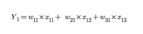
Now, extending this equation to each and every neuron(blue) of the hidden layer, we obtain 4 such equations as we have 4 neurons in the hidden layer. The work that has been done till now, only represents 1 training example/row. In order to send our training data all at once into the feed forward function, we will have to use matrices to perform this operation. But the task really is to verify with full confidence that solving(on paper) the above piece of code which includes dot products and element-wise multiplications matches these 4 linear equations we discussed. But this time we will be applying these equations on all the rows of our training data simultaneously.
I hope you enjoyed getting your hands dirty in solving matrices and equations but trust me it is worth spending time on.
Moving further, we define a function which will predict the output class at run time after our model is trained.
def predict(self,X):
   self.layert_1=ReLU(np.dot(X,self.weights1))
   return sigmoid(np.dot(self.layert_1,self.weights2))
This is the last function in the ‘Neural_Network’ class and the ‘predict’ function does nothing but normal feed forward using the final optimized weights.
Now that we have defined our class, it is time to actually use it.
#----Defining parameters and instantiating Neural_Network class----#epochs=10000 #Number of training iterations
lr=0.5 # learning rate used in Gradient Descent
n=len(X_test)
m=len(X)nn1=Neural_Network(X_train,Y_train)
#creating an object of Neural_Network class#----------------------Training Starts-----------------------------#
for i in range(epochs):
   nn1.FeedForward()
   y_predict_train=enc.inverse_transform(nn1.output.round())
   y_predict_test=enc.inverse_transform(nn1.predict(X_test).round())
   y_train=enc.inverse_transform(Y_train)
   y_test=enc.inverse_transform(Y_test)
   train_accuracy=(m-np.count_nonzero(y_train-y_predict_train))/m
   test_accuracy=(n-np.count_nonzero(y_test-y_predict_test))/n
   nn1.BackPropogation()
   cost=(1/m)*np.sum(np.square(nn1.y-nn1.output))
   print("Epoch {}/{}  ==============================================================:- ".format(i+1,epochs))#----------------Displaying Final Metrics--------------------------#
print("MSE_Cost: {} , Train_Accuracy: {} , Test_Accuracy: {} ".format(cost,train_accuracy,test_accuracy))
After training for 10000 epochs, the following is the result:
Train accuracy : 0.97777
Test accuracy : 0.9
The results look amazing as compared to other machine learning models when applied to the same problem at hand. This network can be extended to a 3- layer network which will have 2 hidden layers using same concepts. You can also try different optimizers like AdaGrad, Adam etc.
You can access my additional work on the ‘Adult Income Prediction’ dataset which uses a similar neural network in my GitHub repository, the link to which is provided below:
Conclusion
In this post, we started learning the basic architecture of a neural network and went further into the components of a neural network architecture. We also witnessed the mathematics behind the working of the same and got a detailed explanation of application of chain rule and basic calculus in developing equations for back-propagation which is a major part of the training process. Finally, we converted our mathematical concepts and equations into code and implemented a full fledged neural network on the IRIS dataset.
Thanks a lot for reading through the article. I hope you understood each and every aspect of it. Feel free to ask any question in the responses section.