Thoughts and Theory
tdGraphEmbed: Temporal Dynamic Graph-Level Embedding
Using NLP methods to represent a sequence of temporal graphs
In this post I’ll share tdGraphEmbed, a method that leverages the temporal information in graphs in-order to create graph-level representation per graph time step. The model and approach were published and presented in CIKM2020.
So, first, what are temporal dynamic graphs?
Temporal dynamic graphs are graphs whose topology evolves overtime, with nodes and edges added and removed between different time snapshots.

What is the motivation to embed these graphs in a graph-level representation?
The novel task of embedding entire graphs into a single embedding in temporal domains has not been addressed yet. Such embeddings, which encode the entire graph structure, can benefit several tasks including graph classification, graph clustering, graph visualisation and mainly: (1) Temporal graph similarity- given a graph snap-shot, we wish to identify the most similar graph structure to it in the past. Consider, for example, a criminal organisation that has previously committed crimes. We would like to predict if the organisation’ network is preparing for another crime by comparing new patterns to those resulting in past crimes. (2) Temporal anomaly detection and trend analysis- a well studied field in the temporal graph domain, aims to identify anomalies in the graph structure over time. For example, a social network activity that becomes viral at a specific point in time because of apolitical event or a network of a company that has changed its organisation structure (members replacing their roles) can be identified as anomalies.
The main idea behind our paper is learning graph representation per time step in the temporal graphs sequence.

Despite other well known methods, our focus is on the entire graph representation and not the node representation.
Notations
For our task, we assume a temporal dynamic graph which is an ordered sequence of 𝑇 graph snapshots: 𝐺={𝐺1,𝐺2, …,𝐺𝑇}. Each graph snapshot is defined as 𝐺𝑡=(𝑉𝑡,𝐸𝑡) where 𝑉𝑡 and 𝐸𝑡 are the vertices (nodes) and edges of 𝐺𝑡, respectively. Each graph snapshot models the state of the graph during the time interval [𝑡−Δ𝑡,𝑡] for some configurable Δ𝑡.
For example, Facebook friendship network can be represented as a temporal graph with a daily granularity, where each day represents the friendship connections that were formed that day.
Let 𝑉 be the set of all vertices that appear in 𝐺. The subset of vertices 𝑉𝑡 which make up 𝐺𝑡 can therefore be defined as 𝑉𝑡⊆𝑉. The number of vertices in each time step can (and is likely to) be different from previous iterations, meaning that|𝑉𝑡|≠|𝑉𝑡+1|. Our aim is to learn a mapping function that embeds a graph 𝐺𝑡 into a 𝑑-dimensional space. The embedding should include nodes’ evolution over time and the graph’s structure. Moreover, graphs with similar nodes, edges and topology should be embedded at greater proximity to one another than to other graphs.
tdGraphEmbed
We propose tdGraphEmbed that embeds the entire graph at timestamp 𝑡 into a single vector, 𝐺𝑡. To enable the unsupervised embedding of graphs of varying sizes and temporal dynamics, we used techniques inspired by the field of natural language processing (NLP).
Intuitively, with analogy to NLP, a node can be thought of as a word (node2vec analogy), and the entire graph can be thought of as a document.
Our approach main two steps:
1. Transforming a Graph to a Document
Since NLP techniques are inherently designed to embed objects (i.e., documents) of varying sizes, we hypothesise that by modelling each graph as a sequence of sentences, we will be able to achieve the same for graphs. We choose to model the graph’s sentences using random walks.
At each time stamp 𝑡, tdGraphEmbed performs 𝛾 random walks of length 𝐿 from each node in the graph.

A code example that transforms set of graphs to set of documents:
A modification to that setting can be performing random walks across time steps until the current graph timestamp:
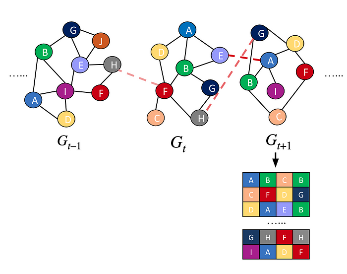
We can use the nodes and edges till the current time t to represent the graph sentences, instead of using only the nodes and edges at time t.
In order to weight the time passed between the current time t and the previous time steps nodes’ connections, we will give the edge a new weight, taking into account that time interval. The new weight for an edge in previous time steps is: w′=w·log(1+1/∆t). Where, w′ is the new weight, w is the previous weight, and ∆t is the time passed between time t and the edge original time. we can use different decay functions of the time interval. This modelling of temporality in the random walks, will help in the current graph representation, by using all the temporal information till that current time.
2. Using Doc2Vec for document embedding
We jointly learn the node embeddings 𝑣 along with the entire graph embedding 𝐺𝑡. Intuitively, instead of using just neighbour nodes to predict the next node in the random walk, as performed by node2vec in static contexts, we extend the CBOW model with additional feature vectors, 𝐺𝑡, which are unique to each graph snapshot, same as Doc2Vec. While the node’s neighbours vectors represent the community of a node, the 𝐺𝑡 graph vectors intend to represent the concept of the entire graph at time 𝑡.
We define the nodes in the neighbourhood of the root node 𝑣𝑖∈𝑉𝑡 as context nodes: 𝑁𝑠(𝑣𝑡𝑖)={𝑣𝑡𝑖−𝜔, …,𝑣𝑡𝑖+𝜔}. The context nodes are of fixed length and sampled from a sliding window 𝜔 over the random walks.
The optimization then becomes predicting a node embedding given the node’s context in the random walks at time 𝑡 of the graph and the vector 𝐺𝑡. Our aim is to maximize the following equation per node 𝑖:
The graph’s time index can be thought of as another node which acts as a memory for the global context of the graph. This global context is combined with the local context of the nodes within the window.
Notice it is a global optimization process through all the time snapshots, i.e., the process enables learning embeddings of the nodes V capturing all the contexts they appear in through the evolution of the graph 𝐺 hand in hand with learning graph vectors for each snapshot 𝐺𝑡. As the model performs random walks through all the time snapshots, it allows modelling graphs with addition and subtraction of nodes over time and does not require a fixed number of nodes for modelling, as static node embedding techniques do. Another advantage of our approach is that it is unsupervised and does not require any task-specific information for its representation learning process. As a result, the produced graph embeddings are generic and can be used in a variety of tasks.
Results
We compared tdGraphEmbed to various baselines, both static and temporal, and on different datasets. We evaluated our method on two main tasks: graph similarity and anomalies and trends detection.
Task 1: Similarity Ranking
In order to evaluate how graph-level embedding generated by tdGraphEmbed captures graph’s similarities, we evaluate our method on graph similarity ranking task. We leverage a commonly used ground truth similarity in graph to graph proximity — Maximum Common Subgraph (MCS). We use cosine similarity metric between the graphs’ vectors generated by each one of the methods. We tested the ranking performance using four measures: Spearman’s Rank CorrelationCoefficient (𝜌), Kendall’s Rank Correlation Coefficient (𝜏),Precision at 10 (p@10), and Precision at 20 (p@20).
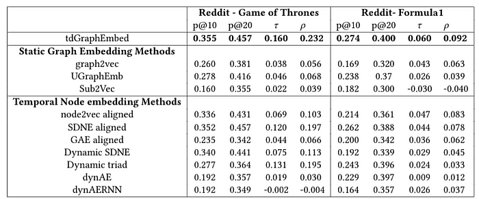

The results in the above tables indicating that our method outperforms the other baselines in capturing graph to graph proximity using MCS.
Task 2: Anomalies and trends detection
Since we deal with temporal graphs embedding we would like to find temporal anomalies in the network. We define anomalies in temporal graph as points in time where the changes to the graph are structural and of a larger scale than average. These changes can be caused by multiple nodes’ changing of communities, the addition/subtraction of nodes, the addition/removal of new edges, etc. We defineΔ𝐺@𝑡 as the change in the graphs’ embedding representation between two consecutive time steps 𝑡−1and 𝑡. Intuitively, values of Δ𝐺@𝑡 that are higher than a predefined threshold value can be used to indicate the existence of anomalies. We defineΔ𝐺@𝑡 using the cosine similarity between the two vectors representing the graphs at time steps 𝑡−1 and 𝑡. We used Precision at 5 (p@5), Precision at 10 (p@10),Recall at 5 (r@5), and Recall at 10 (r@10) to evaluate out the top 5/10 anomalies regarding the ground truth.

Furthermore, we use the graphs embeddings to find trends in the evolutionary networks. To label the trends, we use an external source — Google trends, a popular tool that tracks the popularity of search queries. We calculate the correlation between Google Trends and our embedding trend, Δ𝐺@𝑡 vector using the Spearman correlation measures (𝑠).
As can be shown in the left figures, our method is highly correlated with Google Trends and the anomalous times.


Embedding Visualisation
Visualising the embeddings on a two-dimensional space is a popular way to evaluate node embedding methods. We would like to show that this task is meaningful in the graph-level as well and can be used for graphs clustering. We use TSNE for two-dimensional visualisation of our 128-dimensional graph vectors, where each sample represents a different time granularity. An example on ’Game ofThrones’ dataset, shows that the anomalous days (in red) and consecutive days (examples of this are circled in blue) are close to each other in the two-dimensional space, indicating that our embedding method maintains the characteristics of each time step relative to other similar time steps. It is noteworthy that the anomalous times are located together in the middle of the figure, emphasising that each one of them is close to the days in the same week and to the other anomalous days, since consecutive days share same nodes, but anomalous days share same global structure.

Final Words
(1) tdGraphEmbed, is an unsupervised embedding technique for the entire temporal graph. We jointly learn graph temporal snapshot representations along with node representations. The entire graph snapshot representation is provided by inputting the graph’s time index as an initial input to the context nodes.
(2) We created a dynamic representation, which is capable of modelling a varying number of nodes and edges. Our approach is unsupervised and does not require training data for creating embeddings and can be used for additional tasks.
(3) Our evaluation, conducted on real-world datasets demonstrates that tdGraphEmbed-outperforms many state-of-the-art approaches in graphs’ similarity ranking and detecting temporal anomalies and trends.
Thank you for reading! Feel free to use this work and continue the research at that field.
Our paper

