Self Organizing Maps
(Kohonen’s maps)
Introduction
Self Organizing Maps or Kohenin’s map is a type of artificial neural networks introduced by Teuvo Kohonen in the 1980s. (Paper link)
SOM is trained using unsupervised learning, it is a little bit different from other artificial neural networks, SOM doesn’t learn by backpropagation with SGD,it use competitive learning to adjust weights in neurons. And we use this type of artificial neural networks in dimension reduction to reduce our data by creating a spatially organized representation, also it help us to discover the correlation between data.
SOM’s architecture :
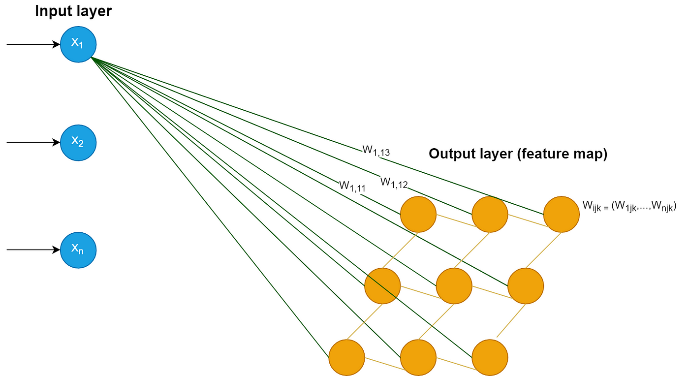
Self organizing maps have two layers, the first one is the input layer and the second one is the output layer or the feature map.
Unlike other ANN types, SOM doesn’t have activation function in neurons, we directly pass weights to output layer without doing anything.
Each neuron in a SOM is assigned a weight vector with the same dimensionality d as the input space.

Self organizing maps training
As we mention before, SOM doesn’t use backpropagation with SGD to update weights, this type of unsupervised artificial neural network uses competetive learning to update its weights.
Competetive learning is based on three processes :
- Competetion
- Cooperation
- Adaptation
Let’s explain those processes.
1)Competetion :
As we said before each neuron in a SOM is assigned a weight vector with the same dimensionality as the input space.
In the example below, in each neuron of the output layer we will have a vector with dimension n.
We compute distance between each neuron (neuron from the output layer) and the input data, and the neuron with the lowest distance will be the winner of the competetion.
The Euclidean metric is commonly used to measure distance.
2) Coorporation:
We will update the vector of the winner neuron in the final process (adaptation) but it is not the only one, also it’s neighbor will be updated.
How do we choose the neighbors ?
To choose neighbors we use neighborhood kernel function, this function depends on two factor : time ( time incremented each new input data) and distance between the winner neuron and the other neuron (How far is the neuron from the winner neuron).
The image below show us how the winner neuron’s ( The most green one in the center) neighbors are choosen depending on distance and time factors.

3) Adaptation:
After choosing the winner neuron and it’s neighbors we compute neurons update. Those choosen neurons will be updated but not the same update, more the distance between neuron and the input data grow less we adjust it like shown in the image below :

The winner neuron and it’s neighbors will be updated using this formula:


This learning rate indicates how much we want to adjust our weights.
After time t (positive infinite), this learning rate will converge to zero so we will have no update even for the neuron winner .

The neighborhood kernel depends on the distance between winner neuron and the other neuron (they are proportionally reversed : d increase make h(t) decrease) and the neighborhood size wich itself depends on time ( decrease while time incrementing) and this make neighborhood kernel function decrease also.
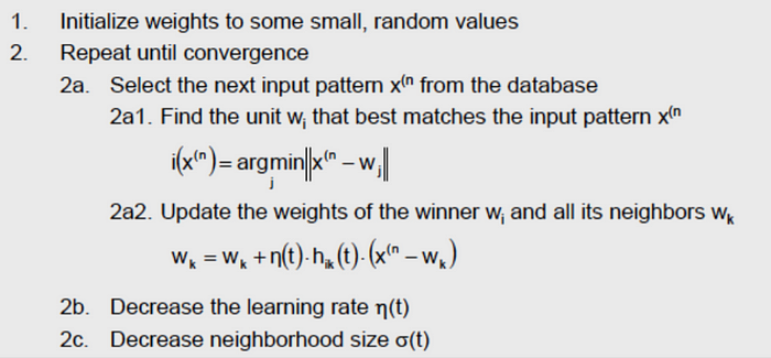
Full SOM algorithm :
Examples :
Let’s see now some examples
Example 1 :

As you can see in this example, feature map take the shape that describe the dataset in 2 dimension space.
Example 2 :