Removing Spikes from Raman Spectra with Anomaly Detection: Whitaker-Hayes algorithm in Python

Abstract. In this article, I would like to comment on a new approach to remove spikes from Raman spectra, presented in the Chemometrics and Intelligent Laboratory Systems journal by D. Whitaker and K. Hayes¹. In their publication, the authors use a modified Z-scores outlier detection based algorithm to locate such spikes, when present, followed by a simple moving average to remove them. Instead of calculating the Z-scores of the spectrum intensity, they calculate the Z-scores of the once-differenced spectrum. They also provided the code for the algorithm implementation in R. Here, I present the implementation of the algorithm in Python and show how I applied it to a different data set.
Raman spectroscopy is a widely used analytical technique which provides structural and electronic information from molecules and solids. It is applicable at both laboratory and mass-production scales, and has applications in many different fields such as physics, chemistry, biology, medicine or industry.
A typical issue known in Raman spectroscopy is that Raman spectra are sometimes ‘contaminated’ by spikes. Spikes are positive, narrow bandwidth peaks present at random position on the spectrum. They originate when a high-energy cosmic ray impacts in the charge-couple device detector used to measure Raman spectra. These spikes are problematic as they might hinder subsequent analysis, particularly if multivariate data analysis is required. Therefore, one of the first steps in the treatment of Raman spectral data is the cleaning of spikes.
First, the Python packages that will be needed are loaded:
import numpy as np
import pandas as pd
import matplotlib.pyplot as plt
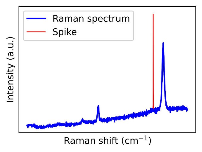
Figure 1 shows the Raman spectrum of graphene. In the previous years, graphene has become a very popular material due to its remarkable physical properties, including superior electronic, thermal, optical and mechanical properties. Its characteristic Raman spectrum consists of several peaks as shown in the figure. From their shape and related intensity, a large amount of information such as doping, strain or grain boundaries can be learned. This spectrum is a clear example of a spectrum contaminated with a spike.
# load the data as data frame
df = pd.read_csv(‘folder_name.../spectrum.txt’, delimiter = ‘\t’)# Transform the data to a numpy array
wavelength = np.array(df.Wavelength)
intensity = np.array(df.Intensity)# Plot the spectrum:
plt.plot(wavelength, intensity)
plt.title(‘Spectrum’, fontsize = 20)
plt.xticks(fontsize = 15)
plt.yticks(fontsize = 15)
plt.xlabel(‘Wavelength (nm)’, fontsize = 20)
plt.ylabel(‘Intensity (a.u.)’, fontsize = 20)
plt.show()

Z-score based approach for spike detection in Raman spectra
Spikes intensities are normally above the intensities of other Raman peaks in the spectrum, therefore using a z-scores based method could be a good starting point. The z-scores tell how far a value is from the average in units of standard deviation. So, if the population mean and population standard deviation are known, the standard score of a raw score x(i) is calculated as:
z(i) = (x(i)-μ) / σ
where μ is the mean and σ is the standard deviation of the population x (x(i) represent the values of a single Raman spectrum). More in detail information on how to detect outliers using Z-score approaches can be found in reference [3].
Let’s calculate the z-scores for the points in our spectrum:
def z_score(intensity):
 mean_int = np.mean(intensity)
 std_int = np.std(intensity)
 z_scores = (intensity — mean_int) / std_int
 return z_scoresintensity_z_score = np.array(z_score(intensity))
plt.plot(wavelength, intensity_z_score)
plt.xticks(fontsize = 15)
plt.yticks(fontsize = 15)
plt.xlabel( ‘Wavelength’ ,fontsize = 20)
plt.ylabel( ‘Z-Score’ ,fontsize = 20)
plt.show()

A threshold is then needed in order to tell whether a value is an outlier or not. A typical value for this threshold is 3.5, as proposed as guideline by the American Society of Quality control as the basis of an outlier-labeling rule², while the authors of the publication used 6. In order to apply a threshold to exclude spikes, the absolute value of the Z-score must be taken:
|z(i)| = |(x(i)-μ) / σ|
calculated as
def z_score(intensity):
 mean_int = np.mean(intensity)
 std_int = np.std(intensity)
 z_scores = (intensity — mean_int) / std_int
 return z_scoresthreshold = 3.5intensity_z_score = np.array(abs(z_score(intensity)))
plt.plot(wavelength, intensity_z_score)
plt.plot(wavelength, threshold*np.ones(len(wavelength)), label = ‘threshold’)
plt.xticks(fontsize = 15)
plt.yticks(fontsize = 15)
plt.xlabel( ‘Wavelength’ ,fontsize = 20)
plt.ylabel( ‘|Z-Score|’ ,fontsize = 20)
plt.show()

However, the z-score pretty much resembles the original spectrum and the threshold still cut off the main Raman peak. Let’s plot what was detected as spikes using a 3.5 threshold:
threshold = 3.5# 1 is assigned to spikes, 0 to non-spikes:
spikes = abs(np.array(z_score(intensity))) > thresholdplt.plot(wavelength, spikes, color = ‘red’)
plt.title(‘Spikes: ‘ + str(np.sum(spikes)), fontsize = 20)
plt.grid()
plt.xticks(fontsize = 15)
plt.yticks(fontsize = 15)
plt.xlabel( ‘Wavelength’ ,fontsize = 20)
plt.ylabel( 'Z-scores > ' + str(threshold) ,fontsize = 20)
plt.show()

Modified Z-score based approach for spike detection in Raman spectra
A second option would be making use of robust statistics and calculate the modified z-scores of the spectrum. This modified Z-score method uses the median (M) and median absolute deviation (MAD) rather than the mean and standard deviation:
z(i) = 0.6745 (x(i)-M) / MAD
where the MAD = median(|x-M|) and |…| represents the absolute value. Both the median and the MAD are robust measures of the central tendency and dispersion, respectively. The multiplier 0.6745 is the 0.75th quartile of the standard normal distribution, to which the MAD converges to⁴.
def modified_z_score(intensity):
 median_int = np.median(intensity)
 mad_int = np.median([np.abs(intensity — median_int)])
 modified_z_scores = 0.6745 * (intensity — median_int) / mad_int
 return modified_z_scoresthreshold = 3.5intensity_modified_z_score = np.array(abs(modified_z_score(intensity)))
plt.plot(wavelength, intensity_modified_z_score)
plt.plot(wavelength, threshold*np.ones(len(wavelength)), label = 'threshold')
plt.xticks(fontsize = 15)
plt.yticks(fontsize = 15)
plt.xlabel('Wavelength (nm)' ,fontsize = 20)
plt.ylabel('|Modified Z-Score|' ,fontsize = 20)
plt.show()

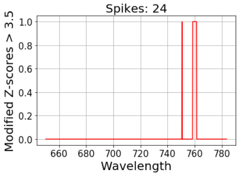
The same issue can still be observed:
# 1 is assigned to spikes, 0 to non-spikes:
spikes = abs(np.array(modified_z_score(intensity))) > thresholdplt.plot(wavelength, spikes, color = ‘red’)
plt.title(‘Spikes: ‘ + str(np.sum(spikes)), fontsize = 20)
plt.grid()
plt.xticks(fontsize = 15)
plt.yticks(fontsize = 15)
plt.xlabel( ‘Wavelength’ ,fontsize = 20)
plt.ylabel( 'Modified Z-scores > ' + str(threshold) ,fontsize = 20)
plt.show()

The 2D Raman peak is still detected as spike, so a more sensitive approach is required.
Whitaker and Hayes’ modified Z-score based approach for spike detection in Raman spectra
Whitaker and Hayes propose to make advantage of the high intensity and small width of spikes and therefore use the difference between consecutive spectrum points ∇x(i) = x(i)-x(i-1) to calculate the z-scores, where x(1), …, x(n) are the values of a single Raman spectrum recorded at equally spaced wavenumbers and i = 2, …, n. This step annihilates linear and slow moving curve linear trends, while sharp thin spikes will be preserved. Now,
z(i) = 0.6745 (∇x(i)-M) / MAD
So there is only an extra step included in which the difference between consecutive values are included.
# First we calculated ∇x(i):
dist = 0
delta_intensity = []
for i in np.arange(len(intensity)-1):
 dist = intensity[i+1] — intensity[i]
 delta_intensity.append(dist)delta_int = np.array(delta_intensity)
# Alternatively to the for loop one can use:
# delta_int = np.diff(intensity)
intensity_modified_z_score = np.array(modified_z_score(delta_int))
plt.plot(wavelength[1:], intensity_modified_z_score)
plt.title('Modified Z-Score using ∇x(i)')
plt.xticks(fontsize = 15)
plt.yticks(fontsize = 15)
plt.xlabel('Wavelength (nm)', fontsize = 20)
plt.ylabel('Score', fontsize = 20)
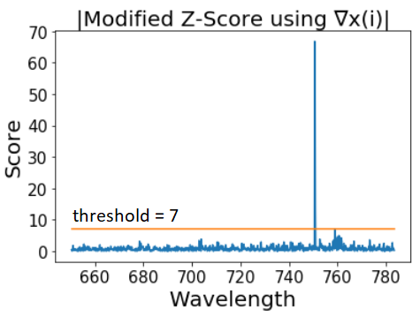
plt.show()

Again, in order to apply a threshold to exclude spikes, the absolute value of the modified Z-score must be taken:
|z(i)| =|0.6745 (∇x(i)-M) / MAD|
Resulting in
threshold = 3.5intensity_modified_z_score = np.array(np.abs(modified_z_score(delta_int)))
plt.plot(wavelength[1:], intensity_modified_z_score)
plt.plot(wavelength[1:], threshold*np.ones(len(wavelength[1:])), label = 'threshold')
plt.title('Modified Z-Score of ∇x(i)', fontsize = 20)
plt.xticks(fontsize = 15)
plt.yticks(fontsize = 15)
plt.xlabel('Wavelength (nm)', fontsize = 20)
plt.ylabel('Score', fontsize = 20)
plt.show()

And once more, the number of detected spikes can be calculated as
# 1 is assigned to spikes, 0 to non-spikes:
spikes = abs(np.array(modified_z_score(intensity))) > thresholdplt.plot(wavelength, spikes, color = ‘red’)
plt.title(‘Spikes: ‘ + str(np.sum(spikes)), fontsize = 20)
plt.grid()
plt.xticks(fontsize = 15)
plt.yticks(fontsize = 15)
plt.xlabel( ‘Wavelength’ ,fontsize = 20)
#plt.ylabel( ‘Spike(1) or not(0)?’ ,fontsize = 20)
plt.show()

For the 3.5 recommended threshold many false spikes are assigned. However, the value scored by this approach is much higher in comparison with the Raman peaks than before.
plt.plot(wavelength[1:],
np.array(abs(modified_z_score(delta_int))), color='black', label = '|Modified Z-Score using ∇x(i)|')
plt.plot(wavelength, np.array(abs(modified_z_score(intensity))), label = '|Modified Z-Score|', color = 'red')
plt.plot(wavelength, np.array(abs(z_score(intensity))), label = '|Z-Score|', color = 'blue')
plt.xticks(fontsize = 15)
plt.yticks(fontsize = 15)
plt.xlabel( 'Wavelength' ,fontsize = 20)
plt.ylabel( 'Score' ,fontsize = 20)
plt.legend()
plt.show()
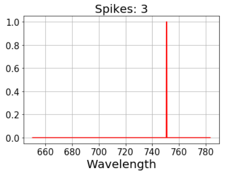
In general, the right threshold must be chosen depending on the data set. For this case, a threshold = 7 is already enough to obtain a clear selection.


Fixing the Raman spectrum
Once the spikes are detected, the next step is to remove them and fix the spectra. For this, interpolated values are obtained at each candidate wavenumber by calculating the mean of its immediate neighbors (within a 2m+1 values window).
def fixer(y,m):
 threshold = 7 # binarization threshold.
 spikes = abs(np.array(modified_z_score(np.diff(y)))) > threshold
 y_out = y.copy() # So we don’t overwrite y for i in np.arange(len(spikes)):
  if spikes[i] != 0: # If we have an spike in position i
   w = np.arange(i-m,i+1+m) # we select 2 m + 1 points around our spike
   w2 = w[spikes[w] == 0] # From such interval, we choose the ones which are not spikes
   y_out[i] = np.mean(y[w2]) # and we average their values

return y_out# Does it work?
plt.plot(wavelength, intensity, label = 'original data')
plt.plot(wavelength, fixer(intensity,m=3), label = 'fixed spectrum')
plt.title('Despiked spectrum',fontsize = 20)
plt.xticks(fontsize = 15)
plt.yticks(fontsize = 15)
plt.xlabel('Wavelength (nm)' ,fontsize = 20)
plt.ylabel('Intensity (a.u.)' ,fontsize = 20)
plt.legend()
plt.show()

So after calculation of the modified Z scores of ∇x, and thresholding by setting an appropiate threshold value, the spike is removed and smoothed by applying a moving average filter.
Other examples
To wrap up, two examples of spikes with different intensity signal are presented, showing the strenght of this approach.

Aknowledgements. I would like to thank Jorge Luis Hita and Ana Solaguren-Beascoa for taking the time to proofread this notes.
[1] Whitaker, Darren A., and Kevin Hayes. “A simple algorithm for despiking Raman spectra.” Chemometrics and Intelligent Laboratory Systems 179 (2018): 82–84.
[2] Iglewicz, B., and D. Hoaglin. “The ASQC basic references in quality control: statistical techniques.” How to detect and handle outliers 16 (1993): 1–87.
[4] Joao Rodrigues. “Outliers make us go MAD: Univariate Outlier Detection”. Medium. https://medium.com/james-blogs/outliers-make-us-go-mad-univariate-outlier-detection-b3a72f1ea8c7


