Reinforcement Learning Concept on Cart-Pole with DQN
A Simple Introduction to Deep Q-Network
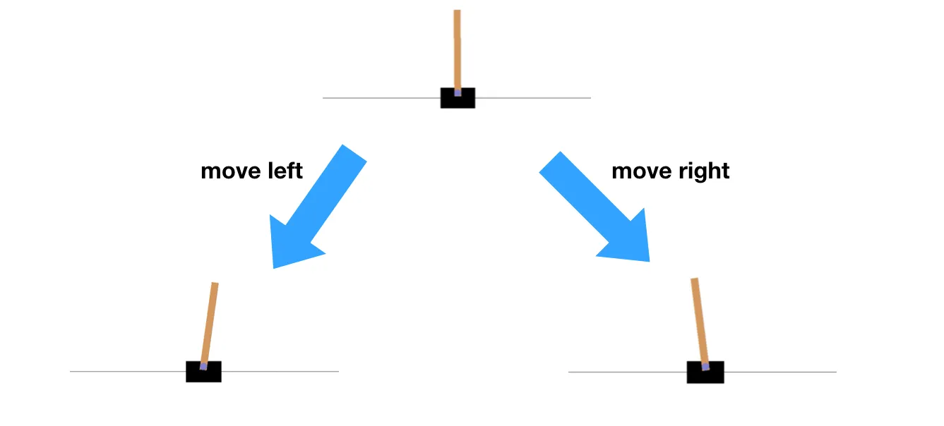
CartPole, also known as inverted pendulum, is a game in which you try to balance the pole as long as possible. It is assumed that at the tip of the pole, there is an object which makes it unstable and very likely to fall over. The goal of this task is to move the cart left and right so that the pole can stand (within a certain angle) as long as possible.

In this post, we will look at reinforcement learning, a field in artificial intelligence where the AI explores the environment all by itself by playing the game many many times until it learns the right way to play the game.

As you can see here, at the beginning of the training, the agent has no idea of where to move a cart. After a while, the agent moves toward a direction but, of course, it is impossible to bring the pole to the other side with such speed. For the last one, the agent knows the correct way to balance the pole which is the move left and right repeatedly.
Rewards
Let’s try to understand this game a little bit more. Again, the objective is to stay alive as long as possible. The longer you keep the pole standing, the more score you will get. This score, also called reward, is what we give to the agent to know if its action is good or not. Based on that, the agent will try to optimize and pick the right action. Note that, the game is over when the pole exceeds 12-degree angle or the cart is going out of the screen.
But how does the agent know the current status of the pole? What should the data look like?
States
The current condition of the cart-pole (of whether it tips over to the left or right) is known as state. A state can be the current frame (in pixels) or it can be some other information that can represent the cart-pole, for instance, the velocity and position of the cart, the angle of the pole and pole velocity at the tip. For this post, let’s assume the state of the cart is the 4 properties mentioned above.
Depending on the action we take, it can lead to different other states. Suppose the pole is starting straight, if we go left, the pole is mostly to go right, which is a new state. Therefore, during each time-step, any action we make will always lead to a different state.
Q-Learning
From the state diagram above, we can see that if we make the right decision, the pole will not fall over and we will get a reward. In other words, for those state and action pairs that lead to further and further states is also expected to get a large reward. So, let’s call this expected reward for each state-action pair as Q-value denoted as Q(s,a).
During a state (s) and the agent takes an action (a), they will immediately get the reward for making that action (1 if the game is still on and 0 otherwise). However, earlier we mentioned that we want to consider the potential future reward of that state-action pair. Let’s consider this case formally with the equation below.

Intuitively, we want to know Q(s,a) which is the expected reward we can get if we are in the state (s) and making (a) action. After getting a reward (r) by making an action (a), we will reach another state (s’). Then, we just look up in our Q table and find the best action to take at state (s’). So, the idea here is we don’t need to consider the entire future actions, but only the one at the next time-step. The gamma symbol (γ) indicates how much we should focus on the future reward of state s’.
At the beginning of the training, we don’t know the Q-value for any state-action pair. Based on the equation above, we can make some changes to Q-value little by little toward a direction of optimal value.

The equation might look a bit terrifying. Don’t worry. We’ll gonna break it down to see what’s going on here with the figure below.

Here, the Q(s,a) will be updated based on the difference between what we think we know about Q(s,a) and what the current episode tell us about Q(s,a) (what it should be). If our Q(s,a) is overestimated, the value in the red dashed box will be negative and we will lower Q(s,a) value by a little. Otherwise, we will increase Q(s,a) value. The amount we make changes to Q(s,a) depends on the difference (red box) and the learning rate (α).
There is one problem with current Q-Learning. That is the state space is huge. Each small change to the angle of the pole or the velocity of the cart represents a new state. We would need to have a very big memory to store all possible states. For this cart-pole, it may be possible to handle that many states but for more complex games like StarCraft 2 or Dota 2, Q-Learning by itself is not enough to get the job done.
Deep Q-Learning
To cope with this problem, we need something to approximate a function that takes in a state-action pair (s,a) and returns the expected reward for that pair. That is when deep learning comes in. It is renowned for approximating a function just from the training data. Keep in mind that we will not go through the detail of the neural network in this post. It will be just a brief on how we can incorporate deep learning with reinforcement learning.

Suppose we want to know Q(s, a=right), we feed in the state (s) of the environment into the model. Let the neural network do the calculation, and it will return 2 values. One is the expected reward when making the left move and another is for making the right move. Since we are interested in a=right, we would just get the value from the lower node of that output. Now we have Q(s,a) by using the network.
To fully train the network, loss function is essential. Intuitively, before the network output an approximated value Q(s,a), we already have an idea of what the value should be (based on equation 2). Hence, we can punish the network for the mistake it makes, and let it learn that mistake through back-propagation.
Putting It Together
Now we have talked about the state, reward, action, Q-learning and DQN specifically on this cart-pole environment. Let’s look at the result of DQN on the cart-pole environment.

Conclusion
So, this is it. We just went through the concept of DQN on a cart-pole game. DQN was successfully applied to many more games especially Atari games. It’s pretty generic and robust. So, next time you have an environment in mind, you can just plug-in DQN and let it learn to play the game by itself. Keep in mind that recently, there are many other deep-reinforcement learning techniques that can learn more complex game like Go or Dota 2 better and faster, but that is the topic for another time.