Random forests and decision trees from scratch in python

Introduction

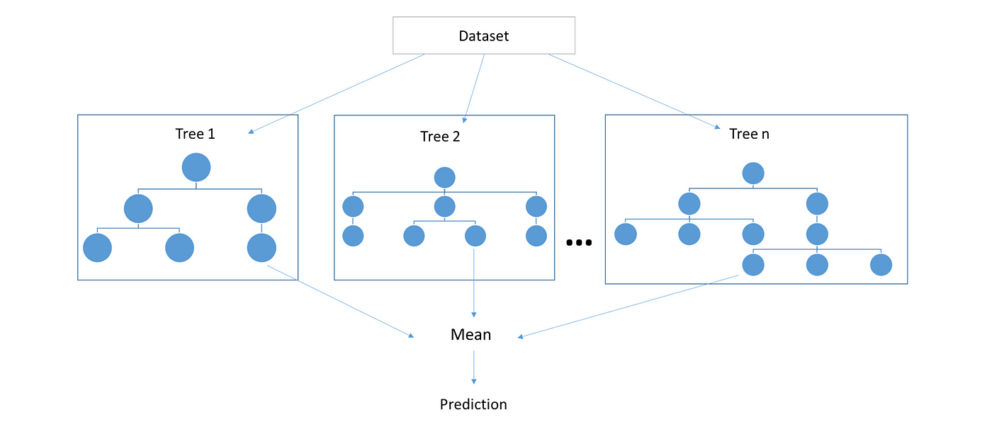
Random forest is the prime example of ensemble machine learning method. In simple words, an ensemble method is a way to aggregate less predictive base models to produce a better predictive model. Random forests, as one could intuitively guess, ensembles various decision trees to produce a more generalized model by reducing the notorious over-fitting tendency of decision trees. Both decision trees and random forests can be used for regression as well as classification problems. In this post we create a random forest regressor although a classifier can be created with little alterations in the following code.

Prerequisites

I advice you to have some working knowledge of the following things to best grasp this post:

1. Decision trees: We will be creating this from scratch too for our random forest but I will not be explaining it’s theory and working mechanism, for brevity facilitates reasoning thus everything mashed up in a single post will only make it unreasonable.
2. Ensemble learning: Random forest is only a subset of this vast set of machine learning technique, you will better understand the post if you have a basic knowledge of this (don’t go into much details only for the sake of this post)
3. numpy and pandas library: A good carpenter must be well versed with his tools. These two libraries are our tools.

Theory

Before starting to write our code, we need to understand some basic theory:

1. Feature bagging: bootstrap aggregating or bagging is a method of selecting a random number of samples from the original set with replacement. In feature bagging the original feature set is randomly sampled and passed onto different trees (without replacement since having redundant features makes no sense). This is done to decrease the correlation among trees. A feature with unmatched great importance will cause every decision tree to choose it for the first and possible consequent splits, this will make all the trees behave similarly and ultimately more correlated which is undesirable. Our aim here is to make highly uncorrelated decision trees.

Why make decision tress highly uncorrelated?

We need highly uncorrelated decision trees because “average error of a bunch of perfectly random errors is zero” hence by decreasing the correlation and making each tree split as randomly as possibly (random in the sense of feature selection, we still aim to find the best split in the randomly selected set of columns), we get better predictions devoid of error.

Correlated trees | Both have same feature set and make similar splits

People travel lands, i travel timeuncorrelated trees | Both have randomly selected different feature set and make different splits

2. Aggregation: The core concept that makes random forests better than decision trees is aggregating uncorrelated trees. The idea is to create several crappy model trees (low depth) and average them out to create a better random forest. Mean of some random errors is zero hence we can expect generalized predictive results from our forest. In case of regression we can average out the prediction of each tree (mean) while in case of classification problems we can simply take the majority of the class voted by each tree (mode).

Python code

To start coding our random forest from scratch, we will follow the top down approach. We will start with a single black box and further decompose it into several black boxes with decreased level of abstraction and greater details until we finally reach a point where nothing is abstracted anymore.

Random forest class

We are creating a random forest regressor, although the same code can be slightly modified to create a classifier. To start out, we need to know what our black box takes as input to yield the output (prediction) so we need to know the parameters that define our random forest :

1. x: independent variables of training set. To keep things minimal and simple I am not creating a separate fit method hence the base class constructor will accept the training set.
2. y: the corresponding dependent variables necessary for supervised learning (Random forest is a supervised learning technique)
3. n_trees : number of uncorrelated trees we ensemble to create the random forest.
4. n_features: the number of features to sample and pass onto each tree, this is where feature bagging happens. It can either be sqrt, log2 or an integer. In case of sqrt, the number of features sampled to each tree is square root of total features and log base 2 of total features in case of log2.
5. sample_size: the number of rows randomly selected and passed onto each tree. This is usually equal to total number of rows but can be reduced to increase performance and decrease correlation of trees in some cases (bagging of trees is a completely separate machine learning technique)
6. depth: depth of each decision tree. Higher depth means more number of splits which increases the over fitting tendency of each tree but since we are aggregating several uncorrelated trees, over fitting of individual trees hardly bothers the whole forest.
7. min_leaf: minimum number of rows required in a node to cause further split. Lower the min_leaf, higher the depth of the tree.

Let’s start defining our random forest class

1. __init__: constructor simply defining the random forest with help of our parameters and creating the required number of trees.
2. create_tree: creates a new decision tree by calling the constructor of class DecisionTree which, for now has been assumed a black box. We will write it’s code later. Each tree receives a random subset of features (feature bagging) and a random set of rows (bagging trees although this is optional I’ve written it to show it’s possibility)
3. predict: our random forest’s prediction is simply the average of all the decision tree predictions.

This is how easy it is to think of a random forest if we can magically create trees. Now we decrease the level of abstraction and write code to create a decision tree.

You can stop reading here if you know how to write a decision tree from scratch but if you don’t then read further.

Decision tree class

It will have the following parameters :-

1. indxs: this parameter exists to keep track of which indices of the original set goes to the right and which goes to the left tree. Hence every tree has this parameter “indxs” which stores the indices of the rows it contains. Prediction is made by averaging these rows.
2. min_leaf: minimum row samples required at a leaf node to be able to cause a split. Every leaf node will have row samples less than min_leaf because they can no more split (ignoring the depth constraint).
3. depth: Max depth or max number of splits possible within each tree.

Why are decision trees only binary?

We’re using the property decorator to make our code more concise.

1. __init__ : the decision tree constructor. It has several interesting snippets to look into:

a. if idxs is None: idxs=np.arange(len(y)) in case we don’t specify the indices of the rows in this particular tree’s calculations, simply take all the rows.

b. self.val = np.mean(y[idxs]) each decision tree predicts a value which is the average of all the rows it’s holding. The variable self.val holds the prediction for each node of the tree. For the root node, the value will simply be the average of all observations because it holds all the rows as we’ve made no split yet. I’ve used the term ‘node’ here because essentially a decision tree is just a node with a decision trees on it’s right and one on it’s left.

c.self.score = float(‘inf’) score of a node is calculated on the basis of how “well” it divides the original data set. We will define this “well” later, lets just assume for now that we have a way to measure such a quantity. Also, the score is set to infinity for our node because we haven’t made any splits yet thus our in-existent split is infinitely bad, indicating that any split will be better than no split.

d. self.find_varsplit() we make our first split!

2. find_varsplit: we use brute force approach to find the best split. This function loops through all the columns sequentially and finds the best split among them all. This function is still incomplete as it only makes a single split, later we extend this function to make left and right decision tree for every split until we reach the leaf node.

3. split_name: A property decorator to return the name of the column we’re splitting over. var_idx is the index of this column, we will calculate this index in the find_better_split function along with value of the column we split upon

4. split_col: A property decorator to return the column at index var_idx with elements at indices given by indxs variable. Basically, segregates a column with selected rows.

5. find_better_split: this functions finds the best possible split in a certain column, it’s a complicated so we’ve considered it as a black box in the above code. Lets define it later.

4. is_leaf: A leaf node is the one that has never made a split thus it has a score of infinite (as mentioned above) hence this functions is used to identify leaf nodes. Also in case we’ve crossed maximum depth i.e. self.depth <= 0, it’s a leaf node as we can’t go any deeper.

How to find the best split?

Decision trees train by splitting the data into two halves recursively based on certain conditions. If a test set has 10 columns with 10 data points (values) in each column, a total of 10x10 = 100 splits are possible, our task in hand is to find which of these splits is the best for our data.

We compare splits based on how well does it split our data into two halves. We make splits such that each of the two half has the most “similar” type of data. One way to increase this similarity is by reducing the variance or standard deviation of both halves. Thus we want to minimize the weighted average (score) of the standard deviation of two halves. We use the greedy approach to find the split by dividing the data into two halves for every value in the column and calculate weighted average (score) of standard deviation of the two halves to ultimately find the minimum. (greedy approach)

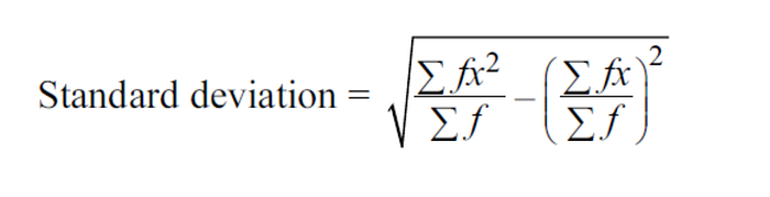
To speed things up, we can make a copy of the column and sort it to calculate the weighted average by splitting over value at n+1th index using the value of sum and sum of squares of values of two halves created by split over nth index. This is based on the following formula of standard deviation :

The following images pictorially showcase the process of score calculations, the last column in each image is a single number representing the score of split i.e weighted average of left and right standard deviations.

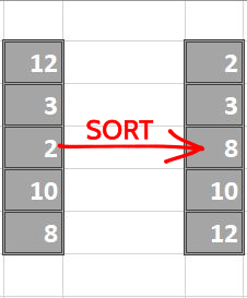
Proceed by sorting each column

Sort the column

Now we make splits index-sequentially

Start with index = 0

index = 1

index = 2 (best split)

index = 3

index = 4

index = 5

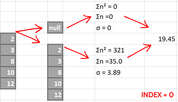
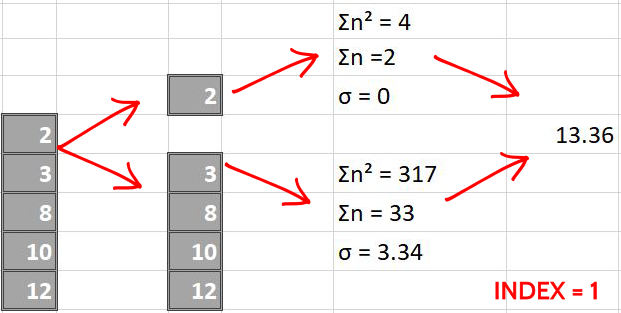
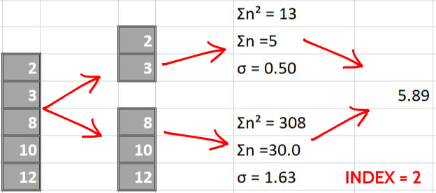
By simple greedy approach, we find that the split made over index = 2 is the best possible split since it has the least score. We perform same steps for all the columns later and compare them all to greedily find the best (minimum) score.

Following is the simple code for above pictorial representations :

The following snippet of code are interesting and need some explanations:

1. function std_agg calculates standard deviation using sum and sum of squares of values
2. curr_score = lhs_std*lhs_cnt + rhs_std*rhs_cnt the split score for each iteration is simply the weighted average of standard deviation of the two halves with number of rows in each half as their weights. Lower score facilitates lower variance, lower variance facilitates grouping of similar data which will lead to better predictions.
3. if curr_score<self.score:
self.var_idx,self.score,self.split = var_idx,curr_score,xi whenever the current score is better (less than the currently saved score in self.score) we will update the current score and store this column in the variable self.var_idx (remember this is the variable that helps selecting the column for two of our property decorators) and save the value upon which the split is made, in the variable self.split .

Now that we know how to find the best split for a chosen column, we need to recursively define splits for each of the further decision trees. For every tree we find the best column and it’s value to split upon then we recursively make two decision trees until we’ve reached the leaf node. To do this, we extend our incomplete function find_varsplit as follows:

1. for i in range(self.c): self.find_better_split(i) this loop goes through every single column and tries to find the best split in that column. By the time this loop ends we’ve exhausted all possible splits over all the columns and found the best possible split. The column to split upon is stored in self.var_idx variable and value of that column we split over is stored in self.split variable. Now we recursively form the two halves i.e. right and left decision trees until we’ve reached the leaf node.
2. if self.is_leaf: return if we’ve reached the leaf node, we no more need to find better splits and simply end this tree.
3. self.lhs holds the left decision tree. The rows it receive are held in lhs which are the indices of all such values in the selected column that are less than or equal to split value stored in split.value . The variable lf_indxs holds the sample of features (columns) the left tree receives (feature bagging).
4. self.rhs holds the right decision tree. rhs stores the indices of rows passed onto the right decision tree. rhs is calculated in a way similar to lhs again, the variable rf_indxs holds the sample of features (columns) the right tree receives (feature bagging).

Conclusion

Here’s the complete code

The intention of this post is to make readers and myself more familiar with the general working of random forests for it’s better application and debugging in future. Random forests have many more parameters and associated complexities that could not be covered in a single post by me. To study a more robust and wholesome code I suggest you read the sklearn module’s random forest code which is open source.

I will like to extend my thanks to Jeremy howard and Rachel thomas for the fast.ai machine learning course which enabled me to write this post. In fact, all of my code here is created after small alterations to the original fast.ai course material.

If I made mistakes / was unclear in my explanations please let me know in the responses. Thank you for reading.