Probability concepts explained: Maximum likelihood estimation

Introduction
In this post I’ll explain what the maximum likelihood method for parameter estimation is and go through a simple example to demonstrate the method. Some of the content requires knowledge of fundamental probability concepts such as the definition of joint probability and independence of events. I’ve written a blog post with these prerequisites so feel free to read this if you think you need a refresher.
What are parameters?
Often in machine learning we use a model to describe the process that results in the data that are observed. For example, we may use a random forest model to classify whether customers may cancel a subscription from a service (known as churn modelling) or we may use a linear model to predict the revenue that will be generated for a company depending on how much they may spend on advertising (this would be an example of linear regression). Each model contains its own set of parameters that ultimately defines what the model looks like.
For a linear model we can write this as y = mx + c. In this example x could represent the advertising spend and y might be the revenue generated. m and c are parameters for this model. Different values for these parameters will give different lines (see figure below).

So parameters define a blueprint for the model. It is only when specific values are chosen for the parameters that we get an instantiation for the model that describes a given phenomenon.
Intuitive explanation of maximum likelihood estimation
Maximum likelihood estimation is a method that determines values for the parameters of a model. The parameter values are found such that they maximise the likelihood that the process described by the model produced the data that were actually observed.
The above definition may still sound a little cryptic so let’s go through an example to help understand this.
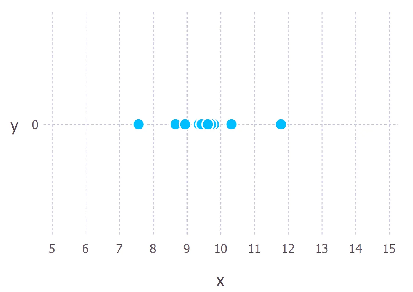
Let’s suppose we have observed 10 data points from some process. For example, each data point could represent the length of time in seconds that it takes a student to answer a specific exam question. These 10 data points are shown in the figure below
We first have to decide which model we think best describes the process of generating the data. This part is very important. At the very least, we should have a good idea about which model to use. This usually comes from having some domain expertise but we wont discuss this here.
For these data we’ll assume that the data generation process can be adequately described by a Gaussian (normal) distribution. Visual inspection of the figure above suggests that a Gaussian distribution is plausible because most of the 10 points are clustered in the middle with few points scattered to the left and the right. (Making this sort of decision on the fly with only 10 data points is ill-advised but given that I generated these data points we’ll go with it).
Recall that the Gaussian distribution has 2 parameters. The mean, μ, and the standard deviation, σ. Different values of these parameters result in different curves (just like with the straight lines above). We want to know which curve was most likely responsible for creating the data points that we observed? (See figure below). Maximum likelihood estimation is a method that will find the values of μ and σ that result in the curve that best fits the data.
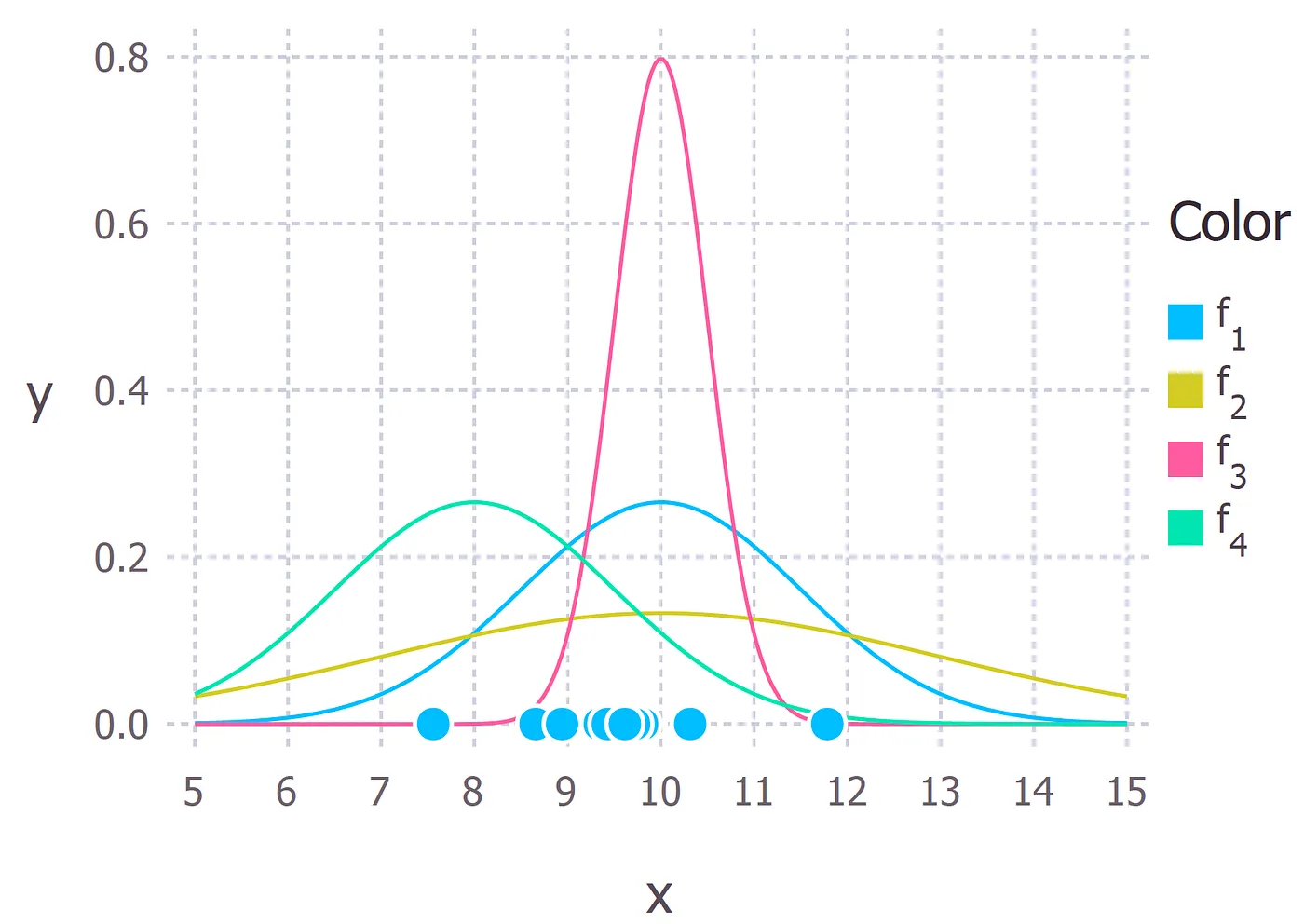
The true distribution from which the data were generated was f1 ~ N(10, 2.25), which is the blue curve in the figure above.
Calculating the Maximum Likelihood Estimates
Now that we have an intuitive understanding of what maximum likelihood estimation is we can move on to learning how to calculate the parameter values. The values that we find are called the maximum likelihood estimates (MLE).
Again we’ll demonstrate this with an example. Suppose we have three data points this time and we assume that they have been generated from a process that is adequately described by a Gaussian distribution. These points are 9, 9.5 and 11. How do we calculate the maximum likelihood estimates of the parameter values of the Gaussian distribution μ and σ?
What we want to calculate is the total probability of observing all of the data, i.e. the joint probability distribution of all observed data points. To do this we would need to calculate some conditional probabilities, which can get very difficult. So it is here that we’ll make our first assumption. The assumption is that each data point is generated independently of the others. This assumption makes the maths much easier. If the events (i.e. the process that generates the data) are independent, then the total probability of observing all of data is the product of observing each data point individually (i.e. the product of the marginal probabilities).
The probability density of observing a single data point x, that is generated from a Gaussian distribution is given by:

The semi colon used in the notation P(x; μ, σ) is there to emphasise that the symbols that appear after it are parameters of the probability distribution. So it shouldn’t be confused with a conditional probability (which is typically represented with a vertical line e.g. P(A| B)).
In our example the total (joint) probability density of observing the three data points is given by:

We just have to figure out the values of μ and σ that results in giving the maximum value of the above expression.
If you’ve covered calculus in your maths classes then you’ll probably be aware that there is a technique that can help us find maxima (and minima) of functions. It’s called differentiation. All we have to do is find the derivative of the function, set the derivative function to zero and then rearrange the equation to make the parameter of interest the subject of the equation. And voilà, we’ll have our MLE values for our parameters. I’ll go through these steps now but I’ll assume that the reader knows how to perform differentiation on common functions. If you would like a more detailed explanation then just let me know in the comments.
The log likelihood
The above expression for the total probability is actually quite a pain to differentiate, so it is almost always simplified by taking the natural logarithm of the expression. This is absolutely fine because the natural logarithm is a monotonically increasing function. This means that if the value on the x-axis increases, the value on the y-axis also increases (see figure below). This is important because it ensures that the maximum value of the log of the probability occurs at the same point as the original probability function. Therefore we can work with the simpler log-likelihood instead of the original likelihood.


Taking logs of the original expression gives us:

This expression can be simplified again using the laws of logarithms to obtain:

This expression can be differentiated to find the maximum. In this example we’ll find the MLE of the mean, μ. To do this we take the partial derivative of the function with respect to μ, giving

Finally, setting the left hand side of the equation to zero and then rearranging for μ gives:

And there we have our maximum likelihood estimate for μ. We can do the same thing with σ too but I’ll leave that as an exercise for the keen reader.
Concluding remarks
Can maximum likelihood estimation always be solved in an exact manner?
No is the short answer. It’s more likely that in a real world scenario the derivative of the log-likelihood function is still analytically intractable (i.e. it’s way too hard/impossible to differentiate the function by hand). Therefore, iterative methods like Expectation-Maximization algorithms are used to find numerical solutions for the parameter estimates. The overall idea is still the same though.
So why maximum likelihood and not maximum probability?
Well this is just statisticians being pedantic (but for good reason). Most people tend to use probability and likelihood interchangeably but statisticians and probability theorists distinguish between the two. The reason for the confusion is best highlighted by looking at the equation.

These expressions are equal! So what does this mean? Let’s first define P(data; μ, σ)? It means “the probability density of observing the data with model parameters μ and σ”. It’s worth noting that we can generalise this to any number of parameters and any distribution.
On the other hand L(μ, σ; data) means “the likelihood of the parameters μ and σ taking certain values given that we’ve observed a bunch of data.”
The equation above says that the probability density of the data given the parameters is equal to the likelihood of the parameters given the data. But despite these two things being equal, the likelihood and the probability density are fundamentally asking different questions — one is asking about the data and the other is asking about the parameter values. This is why the method is called maximum likelihood and not maximum probability.
When is least squares minimisation the same as maximum likelihood estimation?
Least squares minimisation is another common method for estimating parameter values for a model in machine learning. It turns out that when the model is assumed to be Gaussian as in the examples above, the MLE estimates are equivalent to the least squares method. For a more in-depth mathematical derivation check out these slides.
Intuitively we can interpret the connection between the two methods by understanding their objectives. For least squares parameter estimation we want to find the line that minimises the total squared distance between the data points and the regression line (see the figure below). In maximum likelihood estimation we want to maximise the total probability of the data. When a Gaussian distribution is assumed, the maximum probability is found when the data points get closer to the mean value. Since the Gaussian distribution is symmetric, this is equivalent to minimising the distance between the data points and the mean value.

If there is anything that is unclear or I’ve made some mistakes in the above feel free to leave a comment. In the next post I plan to cover Bayesian inference and how it can be used for parameter estimation.
Thank you for reading.