Machine Learning
Predicting Forest Cover Types with the Machine Learning Workflow
a.k.a Fantastic Trees: Where to find, how to detect them 🌲
In this article, I will explain how to approach a multi-class classification supervised machine learning (ML) problem (or project) with an end-to-end workflow.
- Supervised: Features (variables to generate predictions) and target (the variable to be determined) are available in the data set.
- Multi-class classification: There are seven discrete categories to distinguish the target.
Project is based on a famous data set in the machine learning community and known as Forest Cover Type available for download in the UCI Machine Learning Repository.
A stratified sample from the original data set to apply the workflow and separate test set to generate final predictions is used as part of a beginner-friendly competition in Kaggle.
The goal of the Project (and competition): to predict seven different cover types in four different wilderness areas of the Roosevelt National Forest of Northern Colorado with the best accuracy.
Four wilderness areas are:
- 1: Rawah
- 2: Neota
- 3: Comanche Peak
- 4: Cache la Poudre

Seven categories numbered from 1 to 7 in the Cover_Type column, to be classified:
- 1: Spruce/Fir
- 2: Lodgepole Pine
- 3: Ponderosa Pine
- 4: Cottonwood/Willow
- 5: Aspen
- 6: Douglas-fir
- 7: Krummholz
The names of the target (cover type) reminded me of the Fantastic Beasts, so I called them fantastic trees to add some imagination to the project 🙃.
End-to-end Machine Learning Workflow Steps: to classify cover types and reply to the initiating question, where to find fantastic trees and how to detect them, the below steps will be followed:
- Understand, Clean and Format Data
- Exploratory Data Analysis
- Feature Engineering & Selection
- Compare Several Machine Learning Models
- Perform Hyperparameter Tuning on the Best Model
- Interpret Model Results
- Evaluate the Best Model with Test Data (replying the initiating question)
- Summary & Conclusions
I will provide highlights of the project in this article, comprehensive analysis and entire code behind the project is available in the Kaggle notebook and GitHub.
For data wrangling and visualization numpy, pandas, matplotlib, seaborn; for building the machine learning models xgboost, light gbm and scikit-learn; to perform preprocessing steps scikit-learn will be used.
1. Understand, Clean and Format Data
Let’s load the training data and create trees data frame:
trees = pd.read_csv("/kaggle/input/learn-together/train.csv")I always find it useful looking at the first and last rows:


The very first observation is, there are some negative values in the Vertical_Distance_To_Hydrology column. I will examine this in more detail in the Check for Anomalies & Outliers section.
To understand trees dataframe, let’s look at the data types and descriptive statistics. With pandas info method, we can list the non-null values and data types:
Data columns (total 56 columns):
Id                                    15120 non-null int64
Elevation                             15120 non-null int64
Aspect                                15120 non-null int64
Slope                                 15120 non-null int64
Horizontal_Distance_To_Hydrology      15120 non-null int64
Vertical_Distance_To_Hydrology        15120 non-null int64
Horizontal_Distance_To_Roadways       15120 non-null int64
Hillshade_9am                         15120 non-null int64
Hillshade_Noon                        15120 non-null int64
Hillshade_3pm                         15120 non-null int64
Horizontal_Distance_To_Fire_Points    15120 non-null int64
Wilderness_Area1                      15120 non-null int64
Wilderness_Area2                      15120 non-null int64
Wilderness_Area3                      15120 non-null int64
Wilderness_Area4                      15120 non-null int64
Soil_Type1                            15120 non-null int64
Soil_Type2                            15120 non-null int64
Soil_Type3                            15120 non-null int64
Soil_Type4                            15120 non-null int64
Soil_Type5                            15120 non-null int64
Soil_Type6                            15120 non-null int64
Soil_Type7                            15120 non-null int64
Soil_Type8                            15120 non-null int64
Soil_Type9                            15120 non-null int64
Soil_Type10                           15120 non-null int64
Soil_Type11                           15120 non-null int64
Soil_Type12                           15120 non-null int64
Soil_Type13                           15120 non-null int64
Soil_Type14                           15120 non-null int64
Soil_Type15                           15120 non-null int64
Soil_Type16                           15120 non-null int64
Soil_Type17                           15120 non-null int64
Soil_Type18                           15120 non-null int64
Soil_Type19                           15120 non-null int64
Soil_Type20                           15120 non-null int64
Soil_Type21                           15120 non-null int64
Soil_Type22                           15120 non-null int64
Soil_Type23                           15120 non-null int64
Soil_Type24                           15120 non-null int64
Soil_Type25                           15120 non-null int64
Soil_Type26                           15120 non-null int64
Soil_Type27                           15120 non-null int64
Soil_Type28                           15120 non-null int64
Soil_Type29                           15120 non-null int64
Soil_Type30                           15120 non-null int64
Soil_Type31                           15120 non-null int64
Soil_Type32                           15120 non-null int64
Soil_Type33                           15120 non-null int64
Soil_Type34                           15120 non-null int64
Soil_Type35                           15120 non-null int64
Soil_Type36                           15120 non-null int64
Soil_Type37                           15120 non-null int64
Soil_Type38                           15120 non-null int64
Soil_Type39                           15120 non-null int64
Soil_Type40                           15120 non-null int64
Cover_Type                            15120 non-null int64
dtypes: int64(56)
memory usage: 6.5 MB
With describe method, we can observe the descriptive statistics:

info method provided some valuable information:
- Data is formatted and clean: There aren’t any null values and all features are numeric.
- There are one-hot-encoded columns (as verified in the original notebook): Soil type and wilderness area.
Check for Anomalies & Outliers:
The first anomaly was observed with the negative values in the Vertical_Distance_To_Hydrology column. The definition is:
Vertical distance to nearest surface water features
With some research and using logic, negative values show that the nearest surface water is below that data point or it is below the sea level. Either case makes sense, so I am going to keep negative values.
To help future ML model to grasp patterns in the data, I am going to search for outliers and use extreme outliers method to determine them.
Data points will be dropped if they lie more than the 3 times the interquartile range below the first quartile or above the third quartile.
# loop through all columns to see if there are any outliers
for column in trees.columns:
    if outlier_function(trees, column)[2] > 0:
        print("There are {} outliers in {}".format(outlier_function(trees, column)[2], column))
Knowing that the wilderness area and soil type columns are one-hot encoded, we can focus on the rest:
There are 53 outliers in Horizontal_Distance_To_Hydrology
There are 49 outliers in Vertical_Distance_To_Hydrology
There are 3 outliers in Horizontal_Distance_To_Roadways
There are 7 outliers in Hillshade_9am
There are 20 outliers in Hillshade_Noon
There are 132 outliers in Horizontal_Distance_To_Fire_Points
Hillshade columns are the RGB color representation of the shadow at a particular time so the range is already fixed between 0 and 255.
Considering the Horizontal_Distance_To_Firepoints having the highest number of outliers and widest data range [0, 6993], I am going to remove outliers only from that column.
trees = trees[(trees['Horizontal_Distance_To_Fire_Points'] > outlier_function(trees, 'Horizontal_Distance_To_Fire_Points')[0]) &
              (trees['Horizontal_Distance_To_Fire_Points'] < outlier_function(trees, 'Horizontal_Distance_To_Fire_Points')[1])]
2. Exploratory Data Analysis (EDA)
EDA is the first step in this workflow where the decision-making process is initiated for the feature selection. Some valuable insights can be obtained by looking at the distribution of the target, relationship of the features to the target and link between the features.
My preference is to start by looking at the target, then examine the features and its relations to the target.
Distribution of the Target:

Data set have balanced labels, resulting in an almost equal number of cover types for each class. This will be an advantage when we are applying ML algorithms because the model will have a good chance to learn patterns of all classes without needing further balancing strategies.
Wilderness Area — Cover Type:
To have a look at this relationship, wilderness area columns will be reverse-one-hot-encoded.
trees['Wilderness_Area_Type'] = (trees.iloc[:, 11:15] == 1).idxmax(1)
Wilderness area is a distinctive feature for determining the Cover_Type .
Wilderness Area — Soil Type — Cover Type:
Reverse-one-hot-encoding will be applied to soil type columns using the below functions. As a result, one column Soil_Type with discrete numbers between 1 and 40 will be added.

Different wilderness areas consist of some specific trees. Interestingly, there is one fantastic tree, Cottonwood/Willow, specifically likes to grow in Cache la Poudre (Wilderness Area 4). While Spruce/Fir, Lodgepole Pine, Aspen and Douglas-fir can grow in any soil type, other cover types grow with specific soil types.
Relationships Between Continuous Features :
Soil type and wilderness area columns were discrete, and both are the one-hot-encoded version of one categorical feature.
Rest of the features are addressed as continuous: Elevation, Aspect, Slope, Horizontal_Distance_To_Hydrology, Vertical_Distance_To_Hydrology, Horizontal_Distance_To_Roadways, Hillshade_9am, Hillshade_Noon, Hillshade_3pm, Horizontal_Distance_To_Fire_Points.
To visualize all of them with one function Seaborn’s PairGrid will be plotted to provide the flexibility of adjusting upper and lower diagonal with different plots:

The upper half shows the KDE plot with Pearson coefficients and the lower half shows the scatter plot. The diagonal is the histogram of a particular feature. As expected, hillshade features are collinear:
- Hillshade noon — Hillshade 3 pm
- Hillshade 3 pm — Hillshade 9 am
Those pairs provide the same input to the model, for a better interpretability one of them will be dropped in the Feature Engineering & Selection.
Pearson Coefficients of the Features and Target:
As a last step of the EDA, when Pearson coefficients of the features and targets are observed, only 1% of the one-hot-encoded soil type columns are effective in determining the Cover_Type (not shown in this article but in the notebook here). So they will be excluded and Pearson coefficients will be revisited with the continuous features, one-hot-encoded wilderness areas, Soil_Type and Cover_Type .
continuous_variables = trees.columns[1:11].tolist()wilderness_areas = sorted(trees['Wilderness_Area_Type'].value_counts().index.tolist())all_features_w_label = continuous_variables + wilderness_areas + ["Soil_Type"] + ["Cover_Type"]trees_w_numeric_soil = trees[all_features_w_label]

Dark colours represent a strong correlation. Unfortunately, the last column consists of light colours, resulting in weak Pearson coefficients of the features to the target, in the range of [-0.22, 0.12].
With a label-encoded Soil_Type column there is a stronger correlation with the Cover_Type.
Hillshade_9am has the least importance in determining Cover_Type. Thus, it will be dropped in the following section.
3. Feature Engineering & Selection
Extracting new features based on the existing ones and eliminating features with some methods and algorithms are called feature engineering & selection.
There are horizontal and vertical distance to hydrology features, which blinks for adding the euclidian distance of the two.
trees_w_numeric_soil['Euclidian_Distance_To_Hydrology'] = (trees_w_numeric_soil['Horizontal_Distance_To_Hydrology']**2 + trees_w_numeric_soil['Vertical_Distance_To_Hydrology']**2)**0.5Also, adding linear combinations of the numeric features is a common practice in feature engineering. For some of the numeric features, the mean value of the two variables are added:
trees_w_numeric_soil['Mean_Elevation_Vertical_Distance_Hydrology'] = (trees_w_numeric_soil['Elevation'] + trees_w_numeric_soil['Vertical_Distance_To_Hydrology'])/2trees_w_numeric_soil['Mean_Distance_Hydrology_Firepoints'] = (trees_w_numeric_soil['Horizontal_Distance_To_Hydrology'] + trees_w_numeric_soil['Horizontal_Distance_To_Fire_Points'])/2trees_w_numeric_soil['Mean_Distance_Hydrology_Roadways'] = (trees_w_numeric_soil['Horizontal_Distance_To_Hydrology'] + trees_w_numeric_soil['Horizontal_Distance_To_Roadways'])/2trees_w_numeric_soil['Mean_Distance_Firepoints_Roadways'] = (trees_w_numeric_soil['Horizontal_Distance_To_Fire_Points'] + trees_w_numeric_soil['Horizontal_Distance_To_Roadways'])/2
Another common practice is to perform logarithm and square root transformations to the numeric features. After adding 5 more features, square root transformation is applied to the positive features:
for col in trees_w_numeric_soil.columns:
    if trees_w_numeric_soil[col].min() >= 0:
        if col == 'Cover_Type':
            next
        else:
            trees_w_numeric_soil['sqrt' + col] = np.sqrt(trees_w_numeric_soil[col])
After revisiting the Pearson coefficients, if a newly added feature shows a stronger correlation to the target, it is kept and the originating feature is dropped. Additionally, Hillshade_9am is dropped since it is strongly correlated with Hillshade_3pm.

Final features are:
# final list of features
transformed_features = ['sqrtHorizontal_Distance_To_Hydrology', 'sqrtMean_Distance_Hydrology_Roadways', 'sqrtEuclidian_Distance_To_Hydrology',
'Mean_Elevation_Vertical_Distance_Hydrology', 'Mean_Distance_Firepoints_Roadways', 'Mean_Distance_Hydrology_Firepoints']all_features =  (['Elevation', 'Aspect', 'Slope', 'Vertical_Distance_To_Hydrology', 'Horizontal_Distance_To_Roadways',
'Hillshade_Noon', 'Hillshade_3pm', 'Horizontal_Distance_To_Fire_Points' ] +
wilderness_areas + ['Soil_Type'] + transformed_features)trees_training = trees_w_numeric_soil[all_features]
labels_training = trees_w_numeric_soil["Cover_Type"].as_matrix()
To compare ML models and establish a baseline, trees_training and labels_training data frames are split into training and validation set.
X_train, X_valid, y_train, y_valid = train_test_split(trees_training, labels_training, test_size=0.2, random_state=1)- Training set is used as an input, so that machine learning models can catch the patterns in the features and utilize them to distinguish the target.
- Validation set is used to evaluate the ML model’s performance and quantify its ability to generalize patterns to a new data set.
Creating a Baseline Metric:
Before diving deep into the ML classification algorithms, I am going to calculate a common-sense baseline. A common-sense baseline can be defined as how a person who knows that field would solve the problem without using any ML tricks. It can be calculated with human intuition as well as a dummy or simple algorithm, consisting few lines of code.
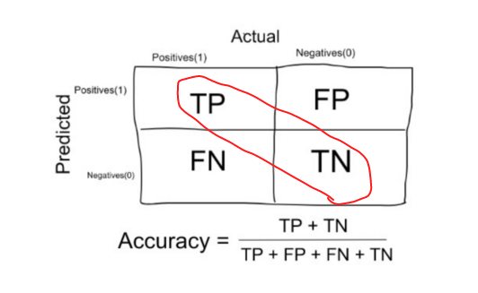
I am going to use a dummy algorithm from the scikit-learn library. With that algorithm, I will establish a baseline metric with accuracy which is the percentage of correctly predicted cover types out of all cover types. Accuracy is the evaluation metric for this competition and will be used throughout the project, keeping in mind that it is not the most effective metric for some classification problems.
Baseline metrics are important in a way that, if a machine learning model can’t beat the simple and intuitive prediction of a person’s or an algorithm’s guess, the original problem needs reconsideration or training data needs reframing.
# Create dummy classifer
dummy = DummyClassifier(strategy='stratified', random_state=1)# train the model
dummy.fit(X_train, y_train)# Get accuracy score
baseline_accuracy = dummy.score(X_valid, y_valid)
print("Our dummy algorithm classified {:0.2f} of the of the trees correctly".format(baseline_accuracy))
Our dummy algorithm classified 0.14 of the of the trees correctly
Now, I expect that following ML models beat the accuracy score of 0.14!
4. Compare Several Machine Learning Models
Sometimes it is hard to know which machine learning model will work effectively for a given problem. So, I always try several machine learning models.
A study shows that tree-based and distance-based algorithms outperform other ML algorithms for the 165 datasets analyzed.

I am going to compare one distance-based algorithm and four tree-based algorithms on accuracy metric.
Distance-based:
- K-Nearest Neighbors Classifier (using euclidian distance to cluster labels; normalization is required before and applied here in the original notebook.)
Tree-based:
- Light Gradient Boosting Machine (LightGBM) Classifier from the light gbm library
- Extra Gradient Boosting (XGBoost) Classifier from the xgboost library
- Random Forest Classifier from the scikit-learn library
- Extra Trees (Random Forests) Classifier from the scikit-learn library
(The code behind the models is here.)
Unlike the study results, extra trees classifier outperformed others. All models beat the baseline-metric showing that machine learning is applicable to the classification of the forest cover types.

Our best model, extra trees classifier, is an ensemble tree-based model. The definition from the scikit-learn library is as follows:
This class implements a meta estimator that fits a number of randomized decision trees (a.k.a. extra-trees) on various sub-samples of the dataset and uses averaging to improve the predictive accuracy and control over-fitting.
The major differences from the random forests algorithm are:
- Rather than looking for a most discriminative split value for a feature in a node, splits are chosen completely randomly as thresholds.
- Sub-samples are drawn from the entire training set instead of a bootstrap sample of the training set.
Thus, the algorithm becomes more robust to over-fitting.
5. Perform Hyperparameter Tuning on the Best Model
Searching for the best combination of model parameters are called hyperparameter tuning which can dramatically improve the model’s performance. I will use the random search algorithm with cross-validation for hyperparameter-tuning:
- Random Search: Set of ML model’s parameters are defined in a range and inputted to sklearn’s
RandomizedSearchCV. This algorithm randomly selects some combination of the parameters and compares the definedscore(accuracy, for this problem) with iterations. Random search runtime and iterations can be controlled with the parametern_iter. - K-Fold Cross-validation: A method used to assess the performance of the hyperparameters on the whole dataset. (visual explanation is here). Rather than splitting the dataset set into two static subsets of training and validation set, data set is divided equally for the given K, and with iterations, different K-1 subsets are trained and model is tested with a different subset.
With the below set of parameters and 5-fold cross-validation RandomizedSearchCV will look for the best combination:
# The number of trees in the forest algorithm, default value is 100.
n_estimators = [50, 100, 300, 500, 1000]

# The minimum number of samples required to split an internal node, default value is 2.
min_samples_split = [2, 3, 5, 7, 9]

# The minimum number of samples required to be at a leaf node, default value is 1.
min_samples_leaf = [1, 2, 4, 6, 8]

# The number of features to consider when looking for the best split, default value is auto.
max_features = ['auto', 'sqrt', 'log2', None]

# Define the grid of hyperparameters to search
hyperparameter_grid = {'n_estimators': n_estimators,
                       'min_samples_leaf': min_samples_leaf,
                       'min_samples_split': min_samples_split,
                       'max_features': max_features}# create model
best_model = ExtraTreesClassifier(random_state=42)

# create Randomized search object
random_cv = RandomizedSearchCV(estimator=best_model,                          param_distributions=hyperparameter_grid,
                               cv=5, n_iter=20,
                               scoring = 'accuracy',
                               n_jobs = -1, verbose = 1,
                               return_train_score = True,
                               random_state=42)# Fit on the all training data using random search object
random_cv.fit(trees_training, labels_training)
random_cv.best_estimator_
Here is the best combination of parameters:
n_estimators= 300max_features= Nonemin_samples_leaf= 1min_samples_split= 2
When I feed them into the extra trees classifier:
Accuracy score in the previous extra random forests model: 0.8659106070713809
Accuracy score after hyperparameter tuning: 0.885923949299533
results in 2 point increase in the accuracy.
Another search method is the GridSearchCV, in contrast to RandomizedSearchCV, the search is performed on every single combination of the given parameters. (applied and discussed here in the original notebook)
6. Interpret Model Results
Confusion Matrix:
One of the most common methods for the visualization of a classification model results is the confusion matrix.
Fantastic tree confusion matrix will be a 7x7 matrix. I will use the normalized confusion matrix, so the percentage of actual cover types correctly guessed out of all guesses in that particular category will appear in the diagonal of the matrix.
Non-diagonal elements will show mislabeled elements by the model. The higher percentages and darker color in the diagonal of the confusion matrix are better, indicating many correct predictions.
I am going to use the function in the scikit-learn to plot it:

The model did pretty good detecting fantastic trees of type Ponderosa Pine, Cottonwood/Willow, Aspen, Douglas-fir, Krummholz, and it seems a bit confused to detect Spruce/Fir and Lodgepole Pine (Cover Type 1 and 2).
Feature Importances:
Another method is to look at the feature importances with feature_importances_: A number between 0 and 1, showing each feature’s contribution to the prediction. Higher the number shows a significant contribution.
With the current selection of features, extra trees classifier and parameters, top 10 features are:

5 of them are created in the scope of this project. This list has stressed the importance of feature engineering and selection.
7. Evaluate the Best Model with Test Data (replying the initiating question)
How to detect fantastic trees (generating final predictions):
Kaggle provides separate training and test set for the competitions. Until now, I worked on the training set. Nonetheless, the test set is used for the final predictions, so I aligned the test set and training set here and fed it into the hyperparameter-tuned Extra Trees Classifier and
successfully detected fantastic trees with 78% accuracy.
Where to find fantastic trees:
Spruce/Fir, Lodgepole Pine and Krummholz love to hangout in Rawah, Neota and Comanche Peak Wilderness Area.
Cache la Poudre Wilderness Area is the perfect place for Ponderosa Pine and Cottonwood/Willow.
If you see an Aspen, suspect that you are at the Rawah or Comanche.
Douglas-fir is an easy-going species, that goes along with any wilderness area.
8. Summary & Conclusions
In this article, I provided highlights of the end-to-end machine learning workflow application to a supervised multi-class classification problem. I started with understanding and visualizing the data with the EDA and formed insights about the cover type dataset. With the outputs of the EDA, I performed feature engineering where I transformed, added and removed features.
Extra trees classifier matched well to this classification problem with the accuracy metric. With the hyperparameter tuning, accuracy score of the model increased by 2 points, by adjusting n_estimators parameter. Interpreting model results showed the most important features and how to improve accuracy further (by distinguishing better between cover type 1 and 2).
For comprehensive code behind the project:
Github Repo: https://github.com/cereniyim/Tree-Classification-ML-Model
Kaggle Notebook: https://www.kaggle.com/cereniyim/fantastic-trees-where-to-find-how-to-detect-them/notebook
