Implementing the Perceptron Algorithm in Python

In this article, we are going to look at the Perceptron Algorithm, which is the most basic single-layered neural network used for binary classification. First, we will look at the Unit Step Function and see how the Perceptron Algorithm classifies and then have a look at the perceptron update rule.

Finally, we will plot the decision boundary for our data. We will use the data with only two features, and there will be two classes since Perceptron is a binary classifier. We will implement all the code using Python NumPy, and visualize/plot using Matplotlib.

Logistic Regression From Scratch in Python

Implementing Polynomial Regression From Scratch in Python

Introduction

The Perceptron algorithm was inspired by the basic processing units in the brain, called neurons, and how they process signals. It was invented by Frank Rosenblatt, using the McCulloch-Pitts neuron and the findings of Hebb. Perceptron Research Paper.

A Perceptron Algorithm is not something widely used in practice. We study it mostly for historical reasons and also because it is the most basic and simple single-layered neural network.

Perceptron

Let us try to understand the Perceptron algorithm using the following data as a motivating example.

from sklearn import datasets

X, y = datasets.make_blobs(n_samples=150,n_features=2,
                           centers=2,cluster_std=1.05,
                           random_state=2)

#Plotting

fig = plt.figure(figsize=(10,8))

plt.plot(X[:, 0][y == 0], X[:, 1][y == 0], 'r^')
plt.plot(X[:, 0][y == 1], X[:, 1][y == 1], 'bs')
plt.xlabel("feature 1")
plt.ylabel("feature 2")
plt.title('Random Classification Data with 2 classes')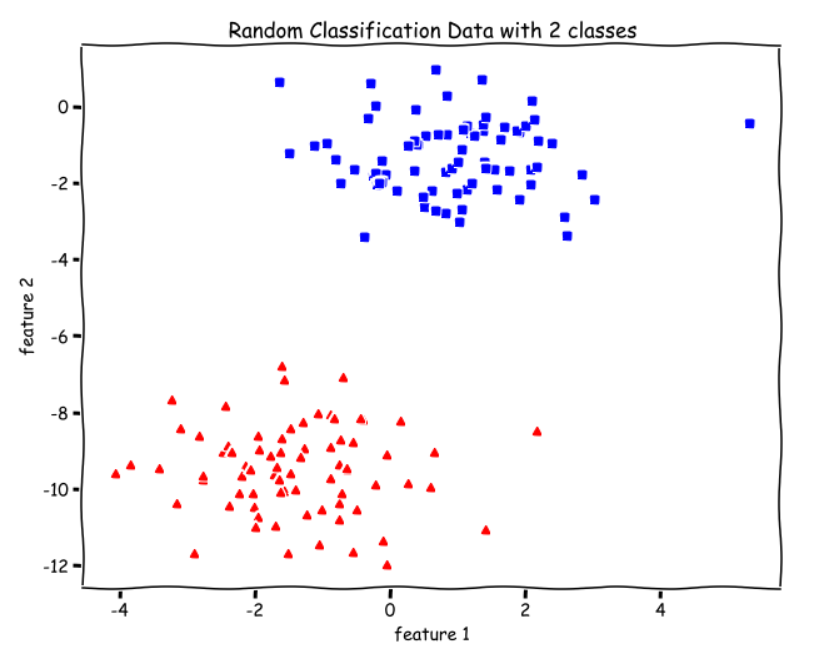

There are two classes, red and green, and we want to separate them by drawing a straight line between them. Or, more formally, we want to learn a set of parameters theta to find an optimal hyperplane(straight line for our data) that separates the two classes.

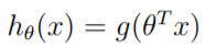
For Linear regression our hypothesis (y_hat) was theta.X. Then, for binary classification in Logistic Regression, we needed to output probabilities between 0 and 1, so we modified the hypothesis as – sigmoid(theta.X). We applied the sigmoid function over the dot product of input features and parameters because we needed to squish our output between 0 and 1.

For the Perceptron algorithm, we apply a different function over theta.X , which is the Unit Step Function, which is defined as –

where,

Unlike Logistic Regression which outputs probability between 0 and 1, the Perceptron outputs values that are either 0 or 1 exactly.

This function says that if the output(theta.X) is greater than or equal to zero, then the model will classify 1(red for example)and if the output is less than zero, the model will classify as 0(green for example). **** And that is how the perception algorithm classifies.

Let’s look at the Unit Step Function graphically –

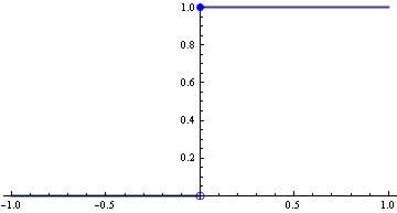
We can see for z≥0, g(z) = 1 and for z<0, g(z) = 0.

Let’s code the step function.

def step_func(z):
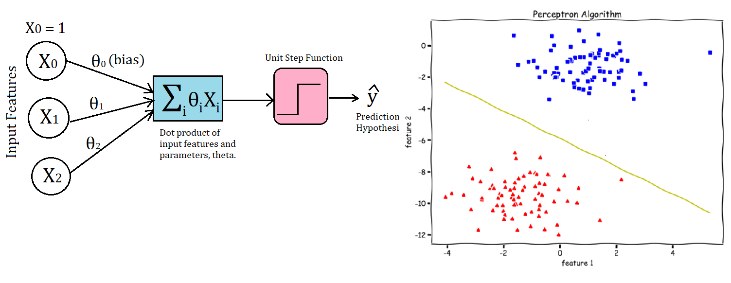
        return 1.0 if (z > 0) else 0.0

Perceptron as a Neural Net

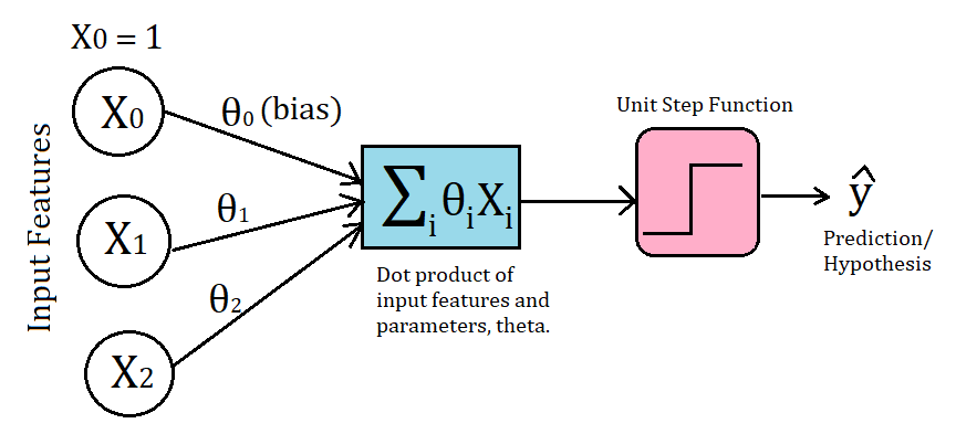
A Perceptron; Image by Author — **A Perceptron**; Image by Author

We can visually understand the Perceptron by looking at the above image. For every training example, we first take the dot product of input features and parameters, theta. Then, we apply the Unit Step Function to make the prediction(y_hat).

And if the prediction is wrong or in other words the model has misclassified that example, we make the update for the parameters theta. We don’t update when the prediction is correct (or the same as the true/target value y).

Let’s see what the update rule is.

Perceptron Update Rule

The perception update rule is very similar to the Gradient Descent update rule. The following is the update rule –

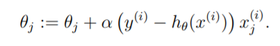
Note that even though the Perceptron algorithm may look similar to logistic regression, it is actually a very different type of algorithm, since it is difficult to endow the perceptron’s predictions with meaningful probabilistic interpretations, or derive the perceptron as a maximum likelihood estimation algorithm.

(From Andrew Ng Course)

Let’s code it. See comments(#).

def perceptron(X, y, lr, epochs):

    # X --> Inputs.
    # y --> labels/target.
    # lr --> learning rate.
    # epochs --> Number of iterations.

    # m-> number of training examples
    # n-> number of features 
    m, n = X.shape

    # Initializing parapeters(theta) to zeros.
    # +1 in n+1 for the bias term.
    theta = np.zeros((n+1,1))

    # Empty list to store how many examples were 
    # misclassified at every iteration.
    n_miss_list = []

    # Training.
    for epoch in range(epochs):

        # variable to store #misclassified.
        n_miss = 0

        # looping for every example.
        for idx, x_i in enumerate(X):

            # Insering 1 for bias, X0 = 1.
            x_i = np.insert(x_i, 0, 1).reshape(-1,1)

            # Calculating prediction/hypothesis.
            y_hat = step_func(np.dot(x_i.T, theta))

            # Updating if the example is misclassified.
            if (np.squeeze(y_hat) - y[idx]) != 0:
                theta += lr*((y[idx] - y_hat)*x_i)

                # Incrementing by 1.
                n_miss += 1

        # Appending number of misclassified examples
        # at every iteration.
        n_miss_list.append(n_miss)

    return theta, n_miss_list

Plotting Decision Boundary

We know that the model makes a prediction of –

_y=1 when y_hat ≥ 0_

_y=0 when y_hat < 0_

So, theta.X = 0 is going to be our Decision boundary.

The following code for plotting the Decision Boundary only works when we have only two features in X.

See comments(#).

def plot_decision_boundary(X, theta):

    # X --> Inputs
    # theta --> parameters

    # The Line is y=mx+c
    # So, Equate mx+c = theta0.X0 + theta1.X1 + theta2.X2
    # Solving we find m and c
    x1 = [min(X[:,0]), max(X[:,0])]
    m = -theta[1]/theta[2]
    c = -theta[0]/theta[2]
    x2 = m*x1 + c

    # Plotting
    fig = plt.figure(figsize=(10,8))
    plt.plot(X[:, 0][y==0], X[:, 1][y==0], "r^")
    plt.plot(X[:, 0][y==1], X[:, 1][y==1], "bs")
    plt.xlabel("feature 1")
    plt.ylabel("feature 2")
    plt.title('Perceptron Algorithm')

    plt.plot(x1, x2, 'y-')

Training and Plotting

theta, miss_l = perceptron(X, y, 0.5, 100)

plot_decision_boundary(X, theta)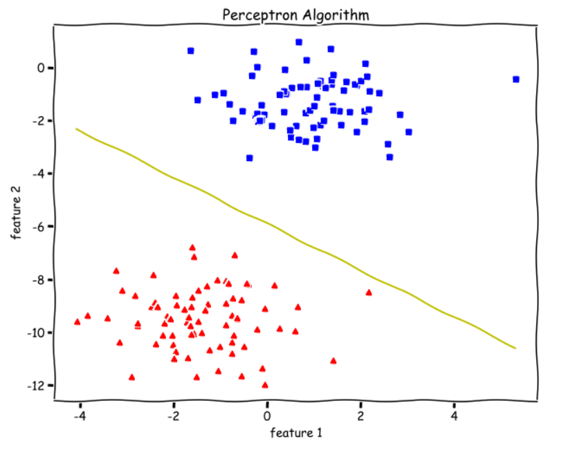

We can see from the above decision boundary graph that we are able to separate the green and blue classes perfectly. Meaning, We get an accuracy of 100%.

Limitations of Perceptron Algorithm

It is only a linear classifier, can never separate data that are not linearly separable.
The algorithm is used only for Binary Classification problems.

Thanks for reading. For questions, comments, concerns, talk to be in the response section. More ML from scratch is coming soon.

Check out the Machine Learning from scratch series –