Generally, multiple linear regression is about quantifying the linear relationship between one dependent variable and several independents variables. By means of this model, we can discover how one variable is influenced by other variables, for example, how income is influenced by education, region, age, gender, etc. However, we need to ask, is the relation shown by the model reliable, or is it spurious?
As an introduction example, to show the importance of examining the partial Correlation, we try to build a multiple linear regression model for income. The dataset is built-in in R and is originally from National Longitudinal Study.
Before building a multivariant model, it’s usually a good practice to examine the correlation first, which is briefly recapped in the next section. We visualize the correlation using the correlation matrix
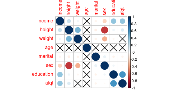
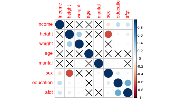
From figure 0.1 we can see that income is positively related to height, weight, education, and afdp (percentile score on Armed Forces Qualification Test); negatively influenced by marital (marital state represented by numbers in the following way: single:1, married:2, separated:3, divorced:4, widowed:5), sex (male represented by one, female two. This negative correlation implies females earn a bit less). The data to some extend confirms what we already know, one thing quite suspicious is that tall people earn more. In fact, this correlation is spurious, and later we will use partial correlation to verify and explain why is it so.
Quick capture of correlation
Correlation describes such relation between two variables, that the growth (decrease) of one of them causes the growth (decrease) of the other.
There are several ways to measure the correlation between two variables. In this post, we use the Pearson correlation coefficient (PCC) also known as Person’s r, since it is also used later in the formula of partial correlation. Another parameter, Spearman’s rho, which is often implemented in R, in fact, uses Person’s r as well, just on top of the rank coefficients. The formula of Person’s r is given by
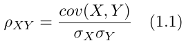
where σₓ is the standard deviation of X, σᵧ is the standard deviation of Y, and cov(X, Y) denotes the covariance, which is defined as the expected value of the product of the deviations of two random variables, X and Y, from their mean, i.e.

correlation normalizes the covariance by dividing it by the standard deviation of the two variables. Unlike covariance, the range of correlation is between -1 and 1. When it equals -1 or 1, it means the relation between the two variables is given exactly be a linear function with positive or negative slope respectively.
Partial correlation – remove the confounder
Partial correlation is a concept closely related to correlation. It shows that fact that when we find a correlation between two variables, this doesn’t necessarily mean that there is causality between them. Partial correlation quantifies the correlation between two variables when conditioned on one or several other variables. This means, when there is a correlation between two variables, the correlation might be partially explained by a third variable – the confounder (or the controlling variable), a common cause of the spurious correlation. After removing this part, what remains, is the partial correlation between those two variables.
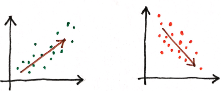
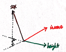
Geometry is one of the intuitive approaches for understanding the partial correlation mentioned in this. Express the variables as vectors, the following figure shows how the confounding factor influences other variables. In our example, the confounding factor is sex, we can see that it is negatively correlated to both income and height.
In the case, where there is only one confounding factor (then it is called a first-order partial correlation), the formula of partial correlation between random variables X and Y with Z factored out is given by

If there are multiple controlling variables, say a set of n controlling variables Z = {Z₁, Z₂, .., Zₙ}, then Z in Eq 2.1 should be replaced by Z which **** denotes a set. The formal definition of partial correlation between X and Y is then
the correlation between the residuals resulting from the linear regression of X with Z and of Y with Z.
In this post, we will stick with the first-order partial correlation. Now we have a different tool in hand, we can revisit our introduction example and investigate the partial correlation between the variables, which is shown in Figure 2.3. This time we can see that height, weight, and marital state are crossed out, compared with the correlation matrix in Figure 0.1.
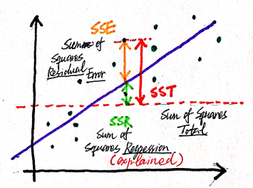
How to compute the partial correlation? Three methods are described on Wikipedia: 1. Linear Regression, 2. recursive formula, 3. matrix inversion. The first method, linear regression, is based on the definition of partial regression, gives us an insight, what are we calculating, when we are calculating the partial correlation. Suppose we want to calculate the partial correlation between X and Y, with the influence of Z removed. The idea is that we first calculate the linear regression of X with regard to Z, and get the residual. Why residual? It is because this is the part in X, which is not explained by Z. And we do this to Y analogously. Then we calculate the correlation between those two residuals. The following illustration shows what "explain" means, it is in fact a term defined in the linear regression
the formal derivation. There is one very important fact worth stressing: (partial) correlation is closely related to linear regression.
We can try to calculate the partial correlation between height and income using regression with the following few lines of code.
m.i <- lm(income ~ sex, data = dataH)
m.s<- lm(height ~ sex, data = dataH)
v.i <- summary(m.i)
v.s <- summary(m.s)
cor(v.i$residuals, v.s$residuals, method="pearson")
The result is 0.094, using linear regression. However, the output of pcor tells us that the partial correlation between height and income is 0.017. Why is it so? It’s because pcor calculated the partial correlation between each pair of variables with the influence of all the other variables removed (using Moore-Penrose generalized matrix inverse). If we take only the subset of the data (only columns income, height, and sex), the output will be the same 0.094.
Apart from helping us identifying the real correlation between two factors in multiple linear regression, partial correlation is also extremely helpful in more complicated models. Autoregressive–moving-average (AMRA) model can serve as such example, where partial correlation, more precisely partial autocorrelation, plays a significant role in hyperparameter selection.
Summary
The topic begins with an introduction example, which shows us that sometimes correlation doesn’t necessarily have to indicate causality. Then we introduce a common cause of this phenomenon – confounding factor, and a way to address this problem – examining the partial correlation. The methods of calculating the partial correlation are also introduced, and the implementation of calculating the partial correlation in R using linear regression is shown.
Resources
[1]Everitt, B. S., & Skrondal, A. The Cambridge dictionary of Statistics (2010).
[2]Kenett, D. Y., Huang, X., Vodenska, I., Havlin, S., & Stanley, H. E. Partial correlation analysis: Applications for financial markets (2015). Quantitative Finance, 15(4), 569–578.