Improve Warehouse Productivity using a Pathfinding Algorithm with Python
Implement a Pathfinding Algorithm with Google AI Operation Research Python Libraries.
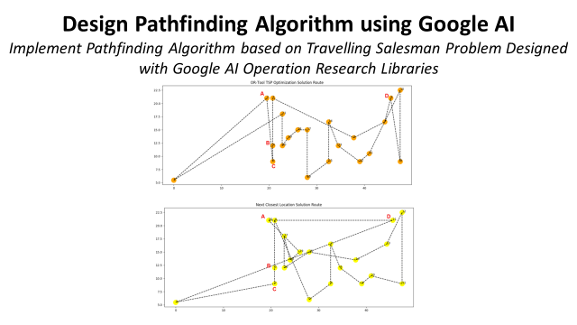
In the highly competitive field of logistics, reducing costs through process optimization is critical.
Among the variable costs of handling goods, order picking is a significant area for cost reduction, mainly influenced by the walking distance covered by operators.
As data scientists, can we leverage path finding algorithms with Python to maximize warehouse picking productivity?
In this series of articles, we started by exploring grouping orders in batches and then introduced spatial clusters of locations picked together.
How many additional productivity points can you earn by implementing pathfinding algorithms with Python?
This article will now focus on designing a pathfinding function with Python to find a sequence of locations to minimize walking distance for warehouse picking.
I. Beyond the Next Closest Location Strategy
  1. Introduction of the model
  2. Limiting Factor: Next Closest Location Strategy
II. Travelling Salesman Problem Application
  1. Google OR-Tools Solutions
  2. OR-Tool Solution vs. Closest Next Location
III. Understand TSP Solution
  1. Highest Gap: 60 m for 21 Picking Locations
  2. Limits of Next Closest Location (NCL) Algorithm
IV. Conclusion
  1. Container Loading Optimization with Python
  2. Impact on your ESG scoring
How to Improve the Picking Path?
Introduction of the model
In the first article, we built a model to test several strategies of Orders Wave Creations to reduce the walking distance.
We started with Warehouse Mapping.

We can link an order line with each picking location's associated warehouse location coordinate (x, y).
We added functions to calculate distances.

This function calculates the walking distance from two locations in the picking path of an operator.
We then added a clustering module.
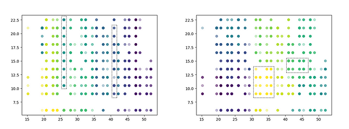
The objective is to group orders by waves using geographical (x, y) clusters to reduce the maximum distance between two locations in the same picking route.
The entire workflow looks like that 👇

At this stage, we have orders grouped by waves to be picked together.
We have a list of picking locations for each wave that the Warehouse Picker must cover.
Limiting Factor: Next Closest Location Strategy
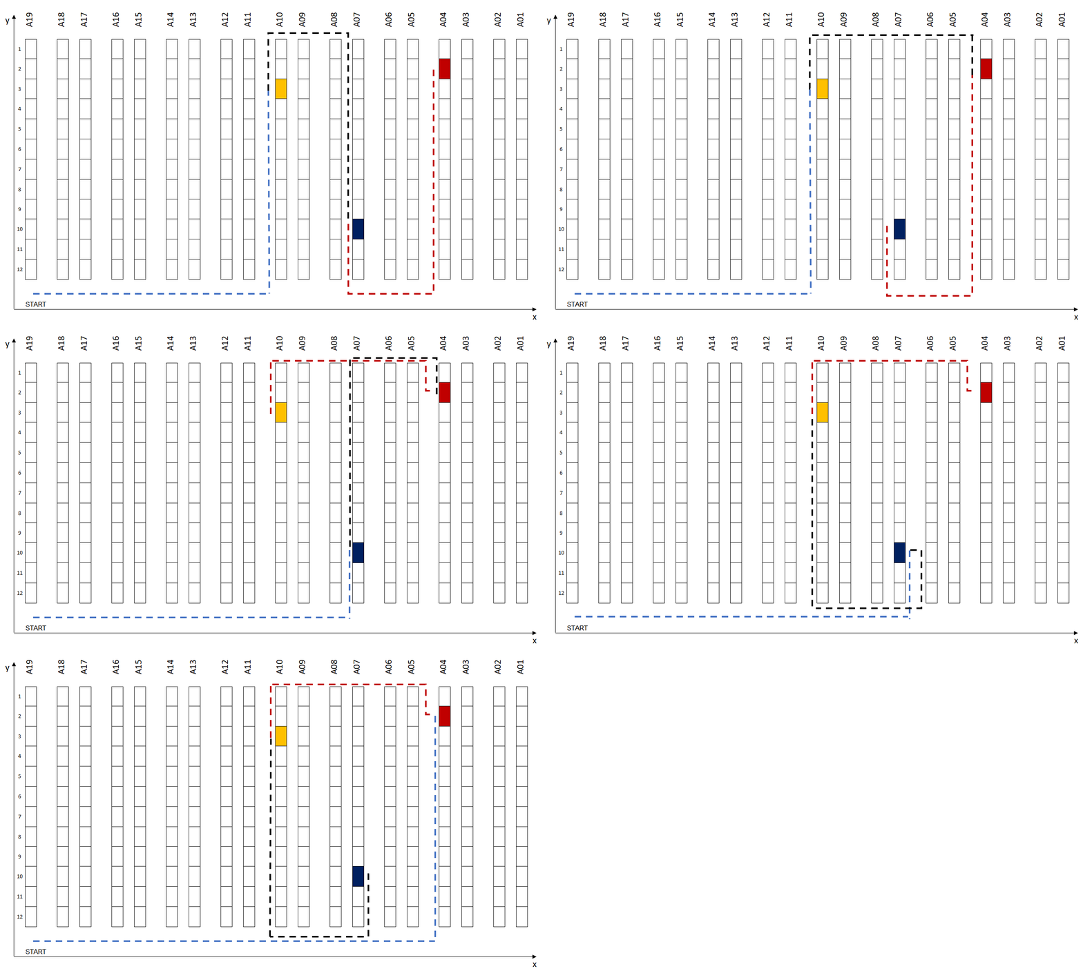
The first article presented an initial solution using the Next Closest Location Strategy.

This simple strategy does not require a high level of computation effort.
From a location j (xj, yj), this function will take as input a list of potential following locations [(xj, yj), (xk, yk), (xh, yh)].
The result will be the closest location, using a custom distance walking function, as the best candidate for the next location to cover.
Is it the most optimal solution for Picking Route Creation ?
While useful, the Next Closest Location Strategy becomes a bottleneck in maximizing productivity.
The next section highlights its limitations and the need for more advanced solutions.
Travelling Salesman Problem Application
Although the results presented in the previous article were promising, we need to grab additional gains to be satisfied.
Logistic operations constantly faces cost pressures, making daily savings a continual challenge.
We will then explore algorithms for creating picking routes using the Single Picker Routing Problem (SPRP) on a two-dimensional warehouse.
SPRP is a specific application of the general Traveling Salesman Problem (TSP) answering the question:
What is the shortest route that visits each storage location and returns to the depot?
Google OR-Tools Solutions
OR-Tools is an open-source collection of tools for combinatorial optimization.
The objective is to find the best solution out of many possible solutions.
Here, we will adapt their Travelling Salesman Problem use case for our specific problem.
Input Data
- List of picking locations coordinates:
List_Coord = [(xi, yi), (x2, y2), …, (x_n, y_n)] - Walking Distance Function
f: ((x_i, y_i), (x_j, y_j)) -> distance(i,j)
Code
In Google OR’s example, a dictionary is created with:
- Distance Matrix: [distance(i,j) for i in [1, n] for j in [1, n]]
- Number of Vehicles: 1 vehicle for our scenario
- Location for depot = start and end: start = end = List_Coord[0]
How much additional walking distance can we save if we implement this for pathfinding?
OR-Tool Solution vs. Next Closest Location
Let us consider that we keep the same order batching strategy and picking location clustering.
What is the impact on total walking distance if we use Google-OR instead of our initial Next Closest Location Solution?
Assumptions
- Order lines: 20,000 Lines
- Distance Threshold: Maximum distance between two picking locations in each cluster (distance_threshold = 35 m)
- Orders per Wave: orders_number in [1, 9]
For the clustering, we will apply three methods
- Method 1: Clustering is not applied
- Method 2: Clustering applied on single-line orders only
- Method 3: Clustering on single-line orders and centroids of multi-line orders
Have a look at the previous article if you need more details,
What were the previous results?
We have run multiple scenarios with several orders per wave, moving from one to nine orders per wave.

Method 3 (applying clustering to all orders) was the most efficient, with nine orders/Wave reducing the walking distance by 83%.
How much can we reduce walking distance by applying TSP-optimized solutions of Google-OR on top of this?
Let us implement this pathfinding solution with our picking route creation workflow.
Code
We now generate a picking route using
- Next Closest Location: distance_init
- TSP Optimized Solution of Google-OR: distance_or
We calculate the results
- Distance Reduction (%): 100 * (distance_init-distance_or)/distance_init
Results for OR-Tools
Observations
- Google's solution is more impactful when the number of orders per wave increases.
- With clustering applied, the impact of the OR tool is reduced.
[Method 3 vs. Method 1]
What is the best scenario?
It remains (Method 3, 9 orders/Wave) with the highest distance reduction with a slight improvement of 1.23% thanks to Google’s solution.
How can you support operations in implementing this solution?
👉You can find the complete code in my GitHub repository: Link
💡 Follow me on Medium for more articles related to 🏭 Supply Chain Analytics, 🌳 Sustainability and 🕜 Productivity.
Understand TSP Solution
For the optimal scenario, OR-Tool TSP Solution reduces the total Walking Distance by 1.23 %.
Why is it better than the initial next closest location strategy?
Let’s have a look at a specific example to understand.
Highest Gap: 60 m for 21 Picking Locations
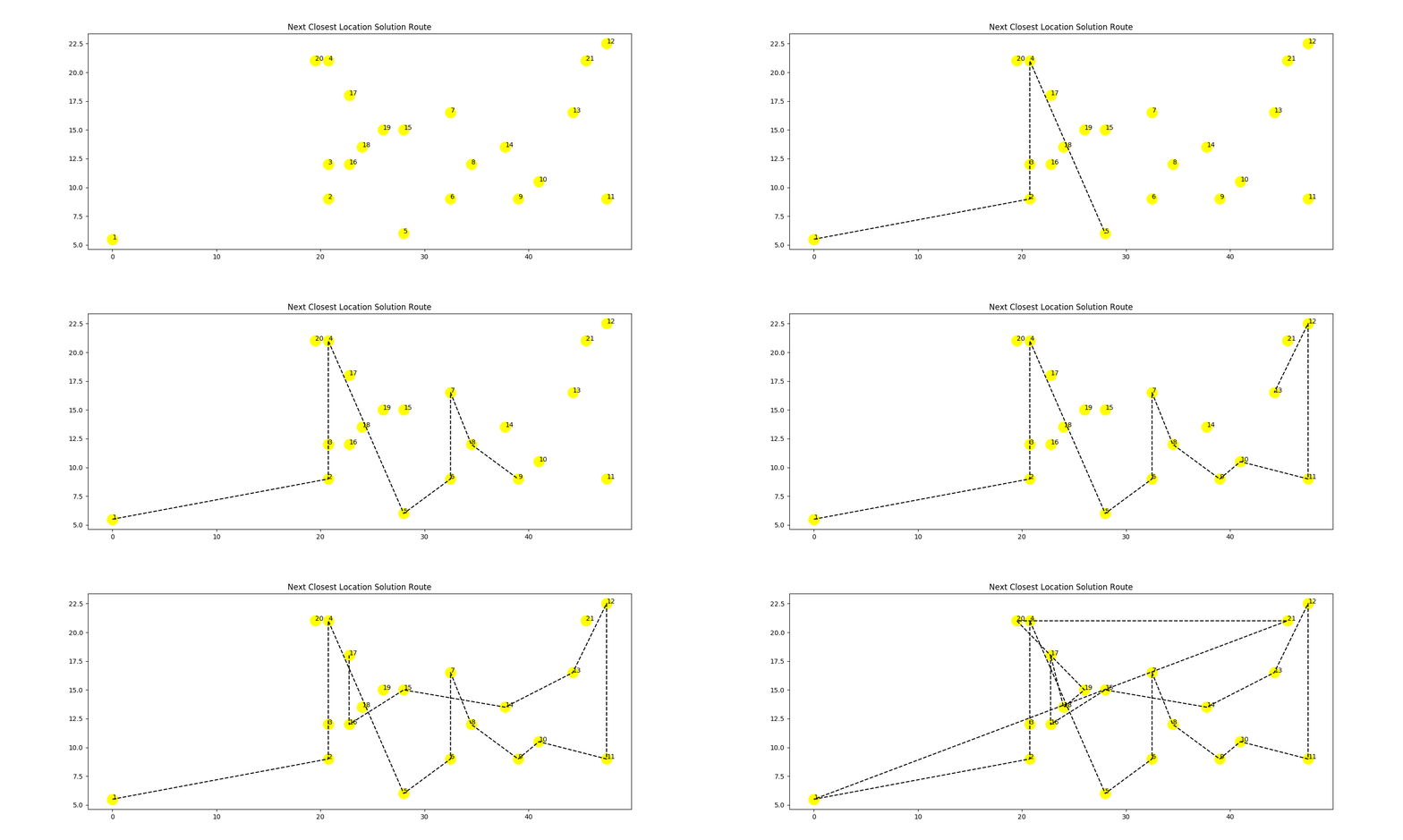
A specific example of one picking wave with 21 Locations covered
- OR-Tool TSP: Distance = 384 m
- Next Closest Location: Distance = 444 m
- Distance Reduction: 60 m

Limits of Next Closest Location (NCL) Algorithm
TSP Point 2 (Point A)
In this specific example, we can see the benefits of the TSP Optimization Solution for the second point (19.5, 21)

Starting at Point 1, the three closest points are {A, B, C}
- The closest point to Point 1 is A
- NCL Point is going directly to C, TSP starts from A
- TSP covers {A, B, C} covers in one time while NCL only covers {B, C} and let A for later

NCL Point 21
In the example above, after Point 20 (Point A), the warehouse picker still needs to cover Point 21 (Point D) before going to the depot (Point 1).
This extra distance significantly impacts NCL's efficiency for this wave.
Do you want to create animated graphs like the one below?

Animate your Python Graphs with Pillow
As asked several times, I shared a simple workflow for generating these Python graph animations in another article.
The approach is straightforward: you generate frames combined in a gif using Python's Pillow library.
For more information, have a look at the article linked below
Conclusion
Applying the Travelling Salesman Problem Solution coupled with intelligent Order Wave Processing can optimize the picking sequence for waves with many picking locations.
You now have a collection of three different layers of optimization you can experiment with your datasets.
- Order batching: group orders in waves
- Spatial clustering: group orders by geographical clusters of Picking Locations to reduce pickers’ walking distance.
- Overcome the next closest location strategy to its limits with Google OR-tool pathfinding solution.
After picking, can we optimize the loading process?
Containers Loading Optimization with Python
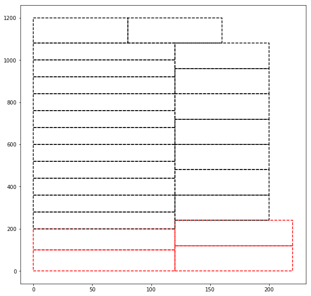
After the container shortage during COVID, optimizing container loading became a priority for logistics teams importing goods from overseas via sea freight.

The example above shows the impact of a wrong loading strategy.
The operator who loaded the left container had two pallets on the side that could not be loaded.
Can we design an algorithm to help forklift drivers maximize the number of pallets loaded per container?
Yes, in another article, I share a case study using an application of the knapsack problem to find the optimal sequence of pallet loading.
For more details, have a look at this article
Beyond reducing costs, these tools benefit operators by allowing them to reach their productivity targets with less effort.
What about the social impact of these algorithms?
Improve ESG Scoring
Environmental, Social and Governance (ESG) reporting is a method companies use to disclose their governance structures, societal impacts and ecological footprint.

As stakeholders increasingly demand corporate social responsibility (CSR), ESG reporting has become critical to companies’ long-term strategies.

The social aspect is essential when we consider productivity and workforce costs.
How can you ensure good working conditions, fair wages and profitability?
The optimization solutions presented in this series of articles can be converted into savings and positive social impacts for the workforce.
- ESG score improvements can be converted into financial gains
- Social aspects gains can improve the reputation of your company
If you want to understand how to convert these gains,
About Me
Let’s connect on Linkedin and Twitter. I am a Supply Chain Engineer who uses data analytics to improve logistics operations and reduce costs.
For consulting or advice on analytics and sustainable supply chain transformation, feel free to contact me via Logigreen Consulting.
If you are interested in Data Analytics and Supply Chain, look at my website.
💌 New articles straight in your inbox for free: Newsletter
📘 Your complete guide for Supply Chain Analytics: Analytics Cheat Sheet
References
[1] Samir Saci, Improve Warehouse Productivity using Order Batching with Python, Link
[2] Samir Saci, Improve Warehouse Productivity using Spatial Clustering for Order Batching with Python Scipy, Link

