One Shot Learning with Siamese Networks using Keras
Table of Contents
- Introduction
- Prerequisites
- Classification vs One Shot Learning
- Applications
- Omniglot Dataset
- Loading the dataset
- Mapping the problem to binary classification task
- Model Architecture and Training
- Validating the Model
- Baseline 1 — Nearest Neighbor Model
- Baseline 2 — Random Model
- Test Results and Inference
- Conclusion
- References
1. Introduction
Deep Convolutional Neural Networks have become the state of the art methods for image classification tasks. However, one of the biggest limitations is they require a lots of labelled data. In many applications, collecting this much data is sometimes not feasible. One Shot Learning aims to solve this problem.
2. Prerequisites
In this post, I will assume that you are already familiar with the basics of machine learning and you have some experience on using Convolutional Neural Networks for image classification using Python and Keras.
3. Classification vs One Shot Learning
In case of standard classification, the input image is fed into a series of layers, and finally at the output we generate a probability distribution over all the classes (typically using a Softmax). For example, if we are trying to classify an image as cat or dog or horse or elephant, then for every input image, we generate 4 probabilities, indicating the probability of the image belonging to each of the 4 classes. Two important points must be noticed here. First, during the training process, we require a large number of images for each of the class (cats, dogs, horses and elephants). Second, if the network is trained only on the above 4 classes of images, then we cannot expect to test it on any other class, example “zebra”. If we want our model to classify the images of zebra as well, then we need to first get a lot of zebra images and then we must re-train the model again. There are applications wherein we neither have enough data for each class and the total number classes is huge as well as dynamically changing. Thus, the cost of data collection and periodical re-training is too high.
On the other hand, in a one shot classification, we require only one training example for each class. Yes you got that right, just one. Hence the name One Shot. Let’s try to understand with a real world practical example.
Assume that we want to build face recognition system for a small organization with only 10 employees (small numbers keep things simple). Using a traditional classification approach, we might come up with a system that looks as below:

Problems:
a) To train such a system, we first require a lot of different images of each of the 10 persons in the organization which might not be feasible. (Imagine if you are doing this for an organization with thousands of employees).
b) What if a new person joins or leaves the organization? You need to take the pain of collecting data again and re-train the entire model again. This is practically not possible specially for large organizations where recruitment and attrition is happening almost every week.
Now let’s understand how do we approach this problem using one shot classification which helps to solve both of the above issues:

Instead of directly classifying an input(test) image to one of the 10 people in the organization, this network instead takes an extra reference image of the person as input and will produce a similarity score denoting the chances that the two input images belong to the same person. Typically the similarity score is squished between 0 and 1 using a sigmoid function; wherein 0 denotes no similarity and 1 denotes full similarity. Any number between 0 and 1 is interpreted accordingly.
Notice that this network is not learning to classify an image directly to any of the output classes. Rather, it is learning a similarity function, which takes two images as input and expresses how similar they are.
How does this solve the two problems we discussed above?
a) In a short while we will see that to train this network, you do not require too many instances of a class and only few are enough to build a good model.
b) But the biggest advantage is that , let’s say in case of face recognition, we have a new employee who has joined the organization. Now in order for the network to detect his face, we only require a single image of his face which will be stored in the database. Using this as the reference image, the network will calculate the similarity for any new instance presented to it. Thus we say that network predicts the score in one shot.
Don’t worry if the above details seem a bit abstract at the moment, just continue ahead and we will solve a problem in full detail and I promise you will develop an in-depth understanding of the subject matter.
4. Applications
Before we proceed, I would like to mention a few applications of one shot learning in order to motivate you so that you develop more keen interest in understanding this technology.
a. As I have already mentioned about face recognition above, just go to this link wherein the AI Guru Andrew Ng demonstrates how Baidu (the Chinese Search Giant) has developed a face recognition system for the employees in their organization.
b. Read this blog to understand how one shot learning is applied to drug discovery where data is very scarce.
c. In this paper, the authors have used one shot learning to build an offline signature verification system which is very useful for Banks and other Government and also private institutions.
5. Omniglot Dataset
For the purpose of this blog, we will use the Omniglot dataset which is a collection of 1623 hand drawn characters from 50 different alphabets. For every character there are just 20 examples, each drawn by a different person. Each image is a gray scale image of resolution 105x105.
Before I continue, I would like to clarify the difference between a character and an alphabet. In case of English the set A to Z is called as the alphabet while each of the letter A, B, etc. is called a character. Thus we say that the English alphabet contains 26 characters (or letters).
So I hope this clarifies the point when I say 1623 characters spanning over 50 different alphabets.
Let’s look at some images of characters from different alphabets to get a better feel of the dataset.

Thus we have 1623 different classes(each character can be treated as a separate class) and for each class we have only 20 images. Clearly, if we try to solve this problem using the traditional image classification method then definitely we won’t be able to build a good generalized model. And with such less number of images available for each class, the model will easily overfit.
You can download the dataset by cloning this GitHub repository. The folder named “Python” contains two zip files: images_background.zip and images_evaluation.zip. Just unzip these two files.
images_background folder contains characters from 30 alphabets and will be used to train the model, while images_evaluation folder contains characters from the other 20 alphabets which we will use to test our system.
Once you unzip the files, you will see below folders (alphabets) in the images_background folder(used for training purpose):

And you will see below folders (alphabets) in the images_evaluation folder (used for testing purpose):

Notice that we will train the system on one set of characters and then test it on a completely different set of characters which were never used during the training. This is not possible in a traditional classification cycle.
6. Loading the dataset
First we need to load the images into tensors and later use these tensors to provide data in batches to the model.
We use below function to load images into tensors:
To call this function as follows, pass the path of the train directory as the parameter as follows:
X,y,c = loadimgs(train_folder)The function returns a tuple of 3 variables. I won’t go through each line of the code, but I will provide you some intuition what exactly the function is doing by understanding the values it returns. Given this explanation you should be in a good position to understand the above function, once you go through it.
Let’s understand what is present in ‘X’:
X.shape
(964, 20, 105, 105)
This means we have 964 characters (or letters or categories) spanning across 30 different alphabets. For each of this character, we have 20 images, and each image is a gray scale image of resolution 105x105. Hence the shape (964, 20, 105, 105).
Let’s now understand how the labels ‘y’ are populated:
y.shape
(19280, 1)
Total number of images = 964 * 20 = 19280. All the images for one letter have the same label., i.e. The first 20 images have the label 0, the next 20 have the label 1, and so on, … the last 20 images have the label 963.
Finally the last variable ‘c’ stands for categories and it is a dictionary as follows:
c.keys() # 'c' for categoriesdict_keys(['Alphabet_of_the_Magi', 'Anglo-Saxon_Futhorc', 'Arcadian', 'Armenian', 'Asomtavruli_(Georgian)', 'Balinese', 'Bengali', 'Blackfoot_(Canadian_Aboriginal_Syllabics)', 'Braille', 'Burmese_(Myanmar)', 'Cyrillic', 'Early_Aramaic', 'Futurama', 'Grantha', 'Greek', 'Gujarati', 'Hebrew', 'Inuktitut_(Canadian_Aboriginal_Syllabics)', 'Japanese_(hiragana)', 'Japanese_(katakana)', 'Korean', 'Latin', 'Malay_(Jawi_-_Arabic)', 'Mkhedruli_(Georgian)', 'N_Ko', 'Ojibwe_(Canadian_Aboriginal_Syllabics)', 'Sanskrit', 'Syriac_(Estrangelo)', 'Tagalog', 'Tifinagh'])c['Alphabet_of_the_Magi']
[0, 19]c['Anglo-Saxon_Futhorc']
[20, 48]
Since there are 30 different alphabets, this dictionary ‘c’ contains 30 items. The key for each item is the name of the alphabet. The value for each item is a list of two numbers: [low, high], where ‘low’ is the label of the first character in that alphabet and ‘high’ is the label of the last character in that alphabet.
Once we load the train and test images, we save the tensors on the disk in a pickle file, so that we can utilize them later directly without having to load the images again.
7. Mapping the problem to binary classification task
Let’s understand how can we map this problem into a supervised learning task where our dataset contains pairs of (Xi, Yi) where ‘Xi’ is the input and ‘Yi’ is the output.
Recall that the input to our system will be a pair of images and the output will be a similarity score between 0 and 1.
Xi = Pair of images
Yi = 1 ; if both images contain the same character
Yi = 0; if both images contain different characters
Let’s have a better understanding by visualizing the dataset below:

Thus we need to create pairs of images along with the target variable, as shown above, to be fed as input to the Siamese Network. Note that even though characters from Sanskrit alphabet are shown above, but in practice we will generate pairs randomly from all the alphabets in the training data.
The code to generate these pairs and targets is shown below:
We need to call the above function by passing the batch_size and it will return “batch_size” number of image pairs along with their target variables.
We will use the below generator function to generate data in batches during the training of the network.
8. Model Architecture and Training
This code is an implementation of the methodology described in this research paper by Gregory Koch et al. Model architecture and hyper-parameters that I have used are all as described in the paper.
Let’s first understand the architecture on a high level before diving into the details. Below I present an intuition of the architecture.
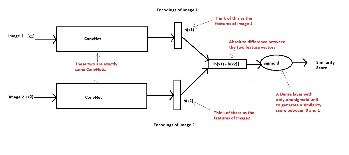
Intuition: The term Siamese means twins. The two Convolutional Neural Networks shown above are not different networks but are two copies of the same network, hence the name Siamese Networks. Basically they share the same parameters. The two input images (x1 and x2) are passed through the ConvNet to generate a fixed length feature vector for each (h(x1) and h(x2)). Assuming the neural network model is trained properly, we can make the following hypothesis: If the two input images belong to the same character, then their feature vectors must also be similar, while if the two input images belong to the different characters, then their feature vectors will also be different. Thus the element-wise absolute difference between the two feature vectors must be very different in both the above cases. And hence the similarity score generated by the output sigmoid layer must also be different in these two cases. This is the central idea behind the Siamese Networks.
Given the above intuition let’s look at the picture of the architecture with more finer details taken from the research paper itself:

The below function is used to create the model architecture:
Notice that there is no predefined layer in Keras to compute the absolute difference between two tensors. We do this using the Lambda layer in Keras which is used to add customized layers in Keras.
To understand the shape of the tensors passed at different layers, refer the below image generated using the plot_model utility of Keras.

The model was compiled using the adam optimizer and binary cross entropy loss function as shown below. Learning rate was kept low as it was found that with high learning rate, the model took a lot of time to converge. However these parameters can well be tuned further to improve the present settings.
optimizer = Adam(lr = 0.00006)
model.compile(loss="binary_crossentropy",optimizer=optimizer)
The model was trained for 20000 iterations with batch size of 32.
After every 200 iterations, model validation was done using 20-way one shot learning and the accuracy was calculated over 250 trials. This concept is explained in the next section.
9. Validating the Model
Now that we have understood how to prepare the data for training, model architecture and training; it’s time we must think about a strategy to validate and test our model.
Note that, for every pair of input images, our model generates a similarity score between 0 and 1. But just looking at the score its difficult to ascertain whether the model is really able to recognize similar characters and distinguish dissimilar ones.
A nice way to judge the model is N-way one shot learning. Don’t worry, it’s much easier than what it sounds to be.
An example of 4-way one shot learning:
We create a dataset of 4 pairs of images as follows:

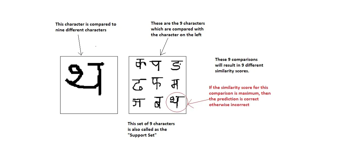
Basically the same character is compared to 4 different characters out of which only one of them matches the original character. Let’s say by doing the above 4 comparisons we get 4 similarity scores S1, S2, S3 and S4 as shown. Now if the model is trained properly, we expect that S1 is the maximum of all the 4 similarity scores because the first pair of images is the only one where we have two same characters.
Thus if S1 happens to be the maximum score, we treat this as a correct prediction otherwise we consider this as an incorrect prediction. Repeating this procedure ‘k’ times, we can calculate the percentage of correct predictions as follows:
percent_correct = (100 * n_correct) / k
where k => total no. of trials and n_correct => no. of correct predictions out of k trials.
Similarly a 9-way one shot learning will look as follows:
A 16-way one shot leaning will be as shown below:

Below is how a 25-way one shot learning would look like:

Note that the value of ’N’ in N-way one shot learning need not necessarily be a perfect square. The reason for me taking values 4, 9, 16 and 25 was because it just looks good for presentation when the square is filled completely.
It’s quite obvious that smaller values of ’N’ will lead to more correct predictions and larger values of ’N’ will lead to relatively less correct predictions when repeated multiple times.
Just a reminder again: All the examples shown above are from the Sanskrit Alphabet but in practice we will generate the test image and the support set randomly from all the alphabets of the test/validation dataset images.
The code to generate the test image along with the support set is as follows:
10. Base Line 1 — Nearest Neighbor Model
It is always a good practice to create simple baseline models and compare their results with complex model you are trying to build.
Our first baseline model is the Nearest Neighbor approach. If you are familiar with K-Nearest Neighbor algorithm, then this is just the same thing.
As discussed above, in an N-way one shot learning, we compare a test image with N different images and select that image which has highest similarity with the test image as the prediction.
This is intuitively similar to the KNN with K=1. Let’s understand in detail how this approach works.
You might have studied how we can compute the L2 distance (also called as the Euclidean distance) between two vectors. If you do not recall, below is how it is done:

Let’s say we compare L2 distance of a vector X with 3 other vectors say A, B and C. Then one way to compute the most similar vector to X is check which vector has the least L2 distance with X. Because distance is inversely proportional to similarity. Thus for example if the L2 distance between X and B is minimum, we say that the similarity between X and B is maximum.
However, in our case we do not have vectors but gray scale images, which can be represented as matrices and not vectors. Then how do we compute L2 distance between matrices?
That’s simple, just flatten the matrices into vectors and then compute the L2 distance between these vectors. For example:

Thus in N-way One Shot learning, we compare the L2 distance of the test image with all the images in the Support Set. Then we check the character for which we got the minimum L2 distance. If this character is the same as the character in the test image, then the prediction is correct, else the prediction is incorrect. For example:

Similar to N way one shot learning, we repeat this for multiple trials and compute the average prediction score over all the trials. The code for nearest neighbor approach is below:
11. Base Line 2 — Random Model
Creating a random model which makes prediction at random is a very common technique to make sure that the model we created is at least better than a model which makes completely random predictions. It’s working can be summarized in the below diagram:

12. Test Results and Inference
The N-way testing was done for N = 1, 3, 5, …., 19.
For each N-way testing, 50 trials were performed and the average accuracy was computed over these 50 trials.
Below is the comparison between the 4 models:

Inference: Clearly the Siamese Model performed much better than the Random Model and the Nearest Neighbor Model. However there is some gap between the results on training set and validation set which indicate that model is over fitting.
13. Conclusion
This is just a first cut solution and many of the hyper parameters can be tuned in order to avoid over fitting. Also more rigorous testing can be done by increasing the value of ’N’ in N-way testing and by increasing the number of trials.
I hope this helped you in understanding the one shot learning methodology using Deep Learning.
Source Code: Please refer my source code in Jupyter Notebook on my GitHub Repository here.
Note: The model was trained on Cloud with a P4000 GPU. If you train it on a CPU, then you need to be very patient.
Comments, suggestions, criticism are welcomed. Thanks.
14. References
a. https://github.com/akshaysharma096/Siamese-Networks
b. https://sorenbouma.github.io/blog/oneshot/
c. https://www.cs.cmu.edu/~rsalakhu/papers/oneshot1.pdf
d. Andrew Ng’s deeplearning.ai Specialization Course on Coursera