ML Algorithms: One SD (σ)
An intro to machine learning algorithms

The obvious questions to ask when facing a wide variety of machine learning algorithms, is “which algorithm is better for a specific task, and which one should I use?”
Answering these questions vary depending on several factors, including: (1) The size, quality, and nature of data; (2) The available computational time; (3) The urgency of the task; and (4) What do you want to do with the data.
In this project I tried to display and briefly explain the main algorithms (though not all of them) that are available for different tasks as simply as possible.
1. Regression Algorithms:

· Ordinary Least Squares Regression (OLSR)- a method in Linear Regression for estimating the unknown parameters by creating a model which will minimize the sum of the squared errors between the observed data and the predicted one (observed values and estimated values).
· Linear Regression- used to estimate real values (cost of houses, number of calls, total sales etc.) based on continuous variable.
· Logistic Regression- used to estimate discrete values ( Binary values like 0/1, yes/no, true/false) based on given set of independent variable
· Stepwise Regression- adds features into your model one by one until it finds an optimal score for your feature set. Stepwise selection alternates between forward and backward, bringing in and removing variables that meet the criteria for entry or removal, until a stable set of variables is attained. Though, I haven’t seen too many articles about it and I heard couple of arguments that it doesn’t work.
· Multivariate Adaptive Regression Splines (MARS) — a flexible regression method that searches for interactions and non-linear relationships that help maximize predictive accuracy. This algorithms is inherently nonlinear (meaning that you don’t need to adapt your model to nonlinear patterns in the data by manually adding model terms (squared terms, interaction effects)).
· Locally Estimated Scatterplot Smoothing (LOESS)- a method for fitting a smooth curve between two variables, or fitting a smooth surface between an outcome and up to four predictor variables. The idea is that what if your data is not linearly distributed you can still apply the idea of regression. You can apply regression and it is called as locally weighted regression. You can apply LOESS when the relationship between independent and dependent variables is non-linear. Today, most of the algorithms (like classical feedforward neural network, support vector machines, nearest neighbor algorithms etc.) are global learning systems where they used to minimize the global loss functions (e.g. sum squared error). In contrast, local learning systems will divide the global learning problem into multiple smaller/simpler learning problems. This usually achieved by dividing the cost function into multiple independent local cost functions. One of the disadvantages of the global methods is that sometimes no parameter values can provide a sufficiently good approximation. But then comes LOESS- an alternative to global function approximation.
2. Instance-based Algorithms:

· K-Nearest Neighbor (KNN) — can be used for both classification and regression problems. KNN stores all available cases and classifies new cases by a majority vote of its K neighbors. Predictions are made for a new data point by searching through the entire training set for the K most similar instances (the neighbors) and summarizing the output variable for those K instances. For regression problems, this might be the mean output variable, for classification problems this might be the mode (or most common) class value.
· Learning Vector Quantization (LVQ) — A downside of K-Nearest Neighbors is that it hangs on to the entire training dataset. LVQ is an artificial neural network algorithm that allows you to choose how many training instances to hang onto and learns exactly what those instances should look like. If you discover that KNN gives good results on your dataset try using LVQ to reduce the memory requirements of storing the entire training dataset.
· Self-Organizing Map (SOM) — an unsupervised deep learning model, mostly used for feature detection or dimensionality reduction. It outputs a 2D map for any number of indicators. SOM differ from other artificial neural networks as it apply competitive learning as opposed to error-correction learning (like backpropagation with gradient descent), and in the sense that they use a neighborhood function to preserve the topological properties of the input space.
· Locally Weighted Learning (LWL) — The idea behind this algorithm is that instead of building a global model for the entire function space, for each point of interest we build a local model based on neighboring data of the query point. For this purpose, each data point becomes a weighting factor which expresses the influence of the data point for the prediction. Mainly, data points that are in the close neighborhood to the current query point are receiving a higher weight than data points which are far away.
3. Regularization Algorithms:

· Ridge Regression (L2 Regularization) — Its goal is to solve problems of data overfitting. A standard linear or polynomial regression model will fail in the case where there is high collinearity (the existence of near-linear relationships among the independent variables) among the feature variables. Ridge Regression adds a small squared bias factor to the variables. Such a squared bias factor pulls the feature variable coefficients away from this rigidness, introducing a small amount of bias into the model but greatly reducing the variance. The Ridge regression has one main disadvantage, it includes all n features in the final model.
· Least Absolute Shrinkage and Selection Operator (LASSO, L1 Regularization) — In opposite to Ridge Regression, it only penalizes high coefficients. Lasso has the effect of forcing some coefficient estimates to be exactly zero when hyper parameter θ is sufficiently large. Therefore, one can say that Lasso performs variable selection producing models much easier to interpret than those produced by Ridge Regression.
· Elastic Net — combines some characteristics from both lasso and ridge. Lasso will eliminate many features, while ridge will reduce the impact of features that are not important in predicting your y values. This algorithm reduces the impact of different features (like ridge) while not eliminating all of the features (like lasso).
· Least-Angle Regression (LARS) — similar to forward stepwise regression. At each step, it finds the predictor most correlated with the response. When multiple predictors having equal correlation exist, instead of continuing along the same predictor, it proceeds in a direction equiangular between the predictors.
4. Decision Tree Algorithms:

· Iterative Dichotomiser 3 (ID3)- builds a tree top-down. It starts at the root and choose an attribute that will be tested at each node. Each attribute is evaluated through some statistical means in order to detect which attribute splits the dataset the best. The best attribute becomes the root, with its attribute values branching out. Then the process continues with the rest of the attributes. Once an attribute is selected, it is not possible to backtrack.
· C4.5 and C5.0 (different versions of a powerful approach) — C4.5, Quinlan’s next iteration is a newer version of ID3. The new features (versus ID3) are: (i) accepts both continuous and discrete features; (ii) handles incomplete data points; (iii) solves over-fitting problem by bottom-up technique usually known as “pruning”; and (iv) different weights can be applied the features that comprise the training data. C5.0, the most recent Quinlan iteration. This implementation is covered by patent and probably as a result, is rarely implemented (outside of commercial software packages).
· Classification and Regression Tree (CART) — CART is used as an acronym for the term decision tree. In general, implementing CART is very similar to implementing the above C4.5. The one difference though is that CART constructs trees based on a numerical splitting criterion recursively applied to the data, while the C4.5 includes the intermediate step of constructing rule sets.
· Chi-squared Automatic Interaction Detection (CHAID) — an algorithm used for discovering relationships between a categorical response variable and other categorical predictor variables. It creates all possible cross tabulations for each categorical predictor until the best outcome is achieved and no further splitting can be performed. CHAID builds a predictive model, or tree, to help determine how variables best merge to explain the outcome in the given dependent variable. In CHAID analysis, nominal, ordinal, and continuous data can be used, where continuous predictors are split into categories with approximately equal number of observations. It is useful when looking for patterns in datasets with lots of categorical variables and is a convenient way of summarizing the data as the relationships can be easily visualized.
· Decision Stump- a ML model that is consisted of a one-level decision tree; a tree with one internal node (the root) which is connected to the terminal nodes (its leaves). This model makes a prediction based on the value of just a single input feature.
· M5- M5 combines a conventional decision tree with the possibility of linear regression functions at the nodes. Besides accuracy, it can take tasks with very high dimension — up to hundreds of attributes. M5 model tree is a decision tree learner for regression task, meaning that it is used to predict values of numerical response variable Y. While M5 tree employs the same approach with CART tree in choosing mean squared error as impurity function, it does not assign a constant to the leaf node but instead it fit a multivariate linear regression model.
5. Bayesian Algorithms:

· Naive Bayes- assumes that the presence of a particular feature in a class is unrelated to the presence of any other feature (independence). Provides a way of calculating posterior probability P(c|x) from P(c), P(x) and P(x|c). Useful for very large data sets.
· Gaussian Naive Bayes- assumes that the distribution of probability is Gaussian (normal). For continuous distributions, the Gaussian naive Bayes is the algorithm of choice.
· Multinomial Naive Bayes — a specific instance of Naive Bayes where the P(Featurei|Class) follows multinomial distribution (word counts, probabilities, etc.). This is mostly used for document classification problem (whether a document belongs to the category of sports, politics, technology etc.). The features/predictors used by the classifier are the frequency of the words present in the document.
· Averaged One-Dependence Estimators (AODE) — developed to address the attribute-independence problem of the naive Bayes classifier. AODE frequently develops considerably more accurate classifiers than naive Bayes with a small cost of a modest increase in the amount of computation.
· Bayesian Belief Network (BBN) — a probabilistic graphical model (a type of statistical model) that represents a set of variables and their conditional dependencies via a directed acyclic graph (DAG). For example, a Bayesian network could represent the probabilistic relationships between diseases and symptoms. Given symptoms, the network can be used to compute the probabilities of the presence of various diseases. A BBN is a special type of diagram (called a directed graph) together with an associated set of probability tables.
· Bayesian Network (BN) — the goal of Bayesian networks is to model conditional dependence, and therefore causation, by representing conditional dependence by edges in a directed graph. Using them, you can efficiently conduct inference on the random variables in the graph through the use of factors.
· Hidden Markov models (HMM) — a class of probabilistic graphical model that give us the ability to predict a sequence of unknown (hidden) variables from a set of observed variables. For example, we can use it to predict the weather (hidden variable) based on the type of clothes that someone wears (observed). HMM can be viewed as a Bayes Net unrolled through time with observations made at a sequence of time steps being used to predict the best sequence of hidden states.
· Conditional random fields (CRFs) — a classical machine learning model to train sequential models. It is a type of Discriminative classifier that model the decision boundary between the different classes. The difference between discriminative and generative models is that while discriminative models try to model conditional probability distribution, i.e., P(y|x), generative models try to model a joint probability distribution, i.e., P(x,y). Their underlying principle is that they apply Logistic Regression on sequential inputs. Hidden Markov Models share some similarities with CRFs, one in that they are also used for sequential inputs. CRFs are most used for NLP tasks.
6. Clustering Algorithms:

· K-Means- a completely differerent algorithm than KNN (don’t confuse the two!). K means goal is to partition X data points into K clusters where each data point is assigned to its closest cluster. The idea is to minimize the sum of all squared distances within a cluster, for all clusters.
· single-linkage clustering- one of several methods of hierarchical clustering. It is based on grouping clusters in bottom-up fashion. In single-linkage clustering, the similarity of two clusters is the similarity of their most similar members.
· K-Medians — a variation of K means algorithm. The idea is that instead of calculating the mean for each cluster (in order to determine its centroid), we calculate the median.
· Expectation Maximization (EM) — it works similarly to K means except for the fact that the data is assigned to each cluster with the weights being soft probabilities instead of distances. It has the advantage that the model becomes generative as we define the probability distribution for each model.
· Hierarchical Clustering- does not partition the dataset into clusters in a single step. Instead it involves multiple steps which run from a single cluster containing all the data points to N clusters containing single data point.
· Fuzzy clustering- a form of clustering in which each data point can belong to more than one cluster.
· DBSCAN (Density-Based Spatial Clustering of Applications with Noise) —used to separate clusters of high density from clusters of low density. DBSCAN requires just two parameters: the minimum distance between two points and the minimum number of points to form a dense region. Meaning, it groups together points that are close to each other (usually Euclidean distance) and a minimum number of points.
· OPTICS (Ordering Points to Identify Cluster Structure) — the idea behind it is similar to DBSCAN, but it addresses one of DBSCAN’s major weaknesses: the problem of detecting meaningful clusters in data of varying density.
· Non negative matrix factorization (NMF) — a Linear-algebraic model that factors high-dimensional vectors into a low-dimensionality representation. Similar to Principal component analysis (PCA), NMF takes advantage of the fact that the vectors are non-negative. By factoring them into the lower-dimensional form, NMF forces the coefficients to also be non-negative.
· Latent Dirichlet allocation (LDA) — a type of probabilistic model and an algorithm used to discover the topics that are present in a corpus. For example, if observations are words collected into documents, to obtain the cluster assignments, it needs two probability values: P( word | topics), the probability of a word given topics. And P( topics | documents), the probability of topics given documents. These values are calculated based on an initial random assignment. Then, you iterate them for each word in each document, to decide their topic assignment.
· Gaussian Mixture Model (GMM) —Its goal is to find a mixture of multi-dimensional Gaussian probability distributions that best model any input dataset. It can be used for finding clusters in the same way that k-means does. The idea is quite simple, find the parameters of the Gaussians that best explain our data. We assume that the data is normal and we want to find parameters that maximize the likelihood of observing these data.
7. Association Rule Learning Algorithms:

· Association rule learning- given a set of transactions, the goal is to find rules that will predict the occurrences of an item based on the occurrences of other items in the transactions.
· Apriori — has great significance in data mining. It is useful in mining frequent itemsets (a collection of one or more items) and relevant association rules. You usually use this algorithm on a database that has a large number of transactions. For example, the items customers buy at a supermarket. The Apriori algorithm reduces the number of candidates with the following principle: If an itemset is frequent, ALL of its subsets are frequent.
· Eclat (Equivalence Class Transformation) — the biggest difference from the Apriori algorithm is that it uses Depth First Search instead of Breadth First Search. In the Apriori algorithm, the element based on the product (shopping cart items 1, 2, 3, 3, etc.) is used, but in Eclat algorithm, the transaction is passed on by the elements (Shopping Cart 100,200 etc.).
· FP (Frequent Pattern) Growth- helps perform a market basket analysis on transaction data. Basically, it’s trying to identify sets of products that are frequently bought together. FP-Growth is preferred to Apriori because Apriori takes more execution time for repeated scanning of the transaction dataset to mine the frequent items.
8. Artificial Neural Network Algorithms:
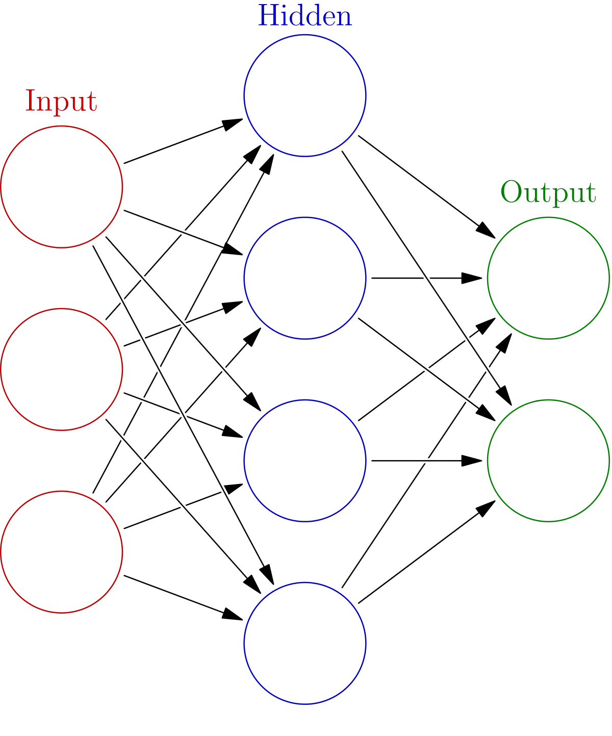
· Perceptron — a single node of a neural network. A perceptron consists of one or more inputs, a processor, and a single output.
· Neural networks — a biologically-inspired method of building computer programs that are able to learn and independently find connections in data.
· Back-Propagation- commonly used by the gradient descent optimization algorithm to adjust the weight of neurons by calculating the gradient of the loss function. I’m keeping it simple here (you should check out the math, it’s quite fascinating)
· Hopfield Network (HN) — HNs are a type of RNN. Their goal is to store 1 or more patterns and to recall the full patterns based on partial input. They are guaranteed to converge to a local minimum (but not necessarily the best one) rather than the stored pattern (expected local minimum). Hopfield nets also provide a model for understanding human memory.
· Autoencoders — used for classification, clustering and feature compression. Autoencoders are unsupervised learning algorithm. The goal of an autoencoder is to learn a representation (encoding) for a set of data, typically for dimensionality reduction, by training the network to ignore signal “noise.”
· Boltzmann machines- a powerful deep learning architecture for collaborative filtering. This model is based on Boltzmann Distribution which is an integral part of statistical mechanics and helps us to understand impact of parameters like temperature and entropy on quantum states in thermodynamics. Boltzmann Machines are mostly divided into two categories: Energy-based Models (EBMs) and Restricted Boltzmann Machines (RBM). When these RBMs are stacked on top of each other, they are known as Deep Belief Networks (DBN).
· Restricted Boltzmann machines (RBM) — neural networks that belong to so called Energy Based Models. RBM is a parameterized generative model representing a probability distribution used to compare the probabilities of (unseen) observations and to sample from the learnt distribution, in particular from marginal distributions of interest.
· Spiking neural nets (SNN) — SNN is fundamentally different from the usual neural networks that people often use. SNNs operate using spikes (which are discrete events that take place at points in time), rather than continuous values. SSN share similarities with how our neurons work. If you consider the membrane potential in our body where once a neuron reaches a certain potential, it spikes, and the potential of that neuron is reset, SSN spike is somewhat similar (except for the fact that the occurrence of a spike is determined by differential equations).
· Radial Basis Function Network (RBFN) — a type of artificial neural network that is used for supervised learning (regression classifications and time series). RBF neural networks are actually FF (feed forward) NNs that use radial basis function as activation function instead of logistic function.
9. Deep Learning Algorithms:

· Deep Boltzmann Machine (DBM) — a type of binary pairwise Markov random field (undirected probabilistic graphical model) with multiple layers of hidden random variables. Unlike Deep Belief Networks (DBN), a DBM is an entirely undirected model. In comparison to fully connected Boltzmann machines (with every unit connected to every other unit), DBM offers advantages similar to those offered by RBM. DBM layers can also be organized as a bipartite graph.
· Deep Belief Networks (DBN) — generative graphical models (a class of deep neural network) composed of multiple layers of latent variables (hidden units), with connections between the layers but not between units within each layer.
· Convolutional Neural Network (CNN) — especially useful for image classification and recognition. They have two main parts: a feature extraction part and a classification part. (See here for more details).
· Stacked Auto-Encoders — a neural network that is consisted of several layers of auto encoders (usually stacked autoencoders look like a “sandwitch”) in which the outputs of each layer is wired to the inputs of the successive layer.
10. Dimensionality Reduction Algorithms:

· Dimensionality reduction- dimensionality reduction algorithm helps us reduce the number of random variables under consideration along with various other algorithms like Decision Tree, Random Forest, PCA, and Factor Analysis.
· Principal Component Analysis (PCA) — a statistical procedure that uses an orthogonal transformation to convert a set of observations of possibly correlated variables into a set of values of linearly uncorrelated variables called principal components. The first component is the most important one, followed by the second, then the third, and so on.
· Independent Component Analysis (ICA) — a statistical technique for revealing hidden factors that underlie sets of random variables, measurements, or signals.
· Principal Component Regression (PCR) — a technique for analyzing multiple regression data that suffer from multicollinearity. The basic idea behind PCR is to calculate the principal components and then use some of these components as predictors in a linear regression model fitted using the typical least squares procedure.
· Partial Least Squares Regression (PLSR) — PCR creates components to explain the observed variability in the predictor variables, without considering the response variable at all. On the other hand, PLSR does take the response variable into account, and therefore often leads to models that are able to fit the response variable with fewer components.
· Sammon Mapping- an algorithm that maps a high-dimensional space to a space of lower dimensionality by trying to preserve the structure of inter-point distances in high-dimensional space in the lower-dimension projection. sometimes we have to ask the question “what non-linear transformation is optimal for some given dataset”. While PCA simply maximizes variance, sometimes we need to maximize some other measure that represents the degree to which complex structure is preserved by the transformation. Various such measures exist, and one of these defines the so-called Sammon Mapping. It is particularly suited for use in exploratory data analysis.
· Multidimensional Scaling (MDS) — a means of visualizing the level of similarity of individual cases of a dataset.
· Projection Pursuit- a type of statistical technique that involves finding the most “interesting” possible projections in multidimensional data. Often, projections which deviate more from a normal distribution are considered to be more interesting.
· Linear Discriminant Analysis (LDA) —if you need a classification algorithm you should start with logistic regression. However, LR is traditionally limited to only two class classification problems. Now, if your problem involves more than two classes you should use LDA. LDA also works as a dimensionality reduction algorithm; it reduces the number of dimension from original to C — 1 number of features where C is the number of classes.
· Mixture Discriminant Analysis (MDA) — It is an extension of linear discriminant analysis. Its a supervised method for classification that is based on mixture models.
· Quadratic Discriminant Analysis (QDA) — Linear Discriminant Analysis can only learn linear boundaries, while Quadratic Discriminant Analysis is capable of learning quadratic boundaries (hence it is more flexible). Unlike LDA however, in QDA there is no assumption that the covariance of each of the classes is identical.
· Flexible Discriminant Analysis (FDA) — a classification model based on a mixture of linear regression models, which uses optimal scoring to transform the response variable so that the data are in a better form for linear separation, and multiple adaptive regression splines to generate the discriminant surface.
11. Ensemble Algorithms:

- Ensemble Methods- learning algorithms that construct a set of classifiers and then classify new data points by taking a weighted vote of their predictions. The original ensemble method is Bayesian averaging, but more recent algorithms include error-correcting output coding, bagging, and boosting.
· Boosting- a family of algorithms which converts weak learner (a classifier that is only slightly correlated with the true classification. Meaning, it can label examples better than random guessing) to strong learners. Using this ensemble method, you can improve the model predictions of any given learning algorithm. The technique fits consecutive trees (random sample), and at every step the goal is to solve for the net error from the prior tree. It is used to primarily reducing bias, and also variance in supervised learning. It basically combines the prediction of several base estimators in order to improve robustness over a single estimator (it combines multiple weak or average predictors to a build strong predictor).
· Bootstrapped Aggregation (Bagging)-used when our goal is to reduce the variance of a decision tree. The idea is to create several subsets of data from training sample chosen randomly with replacement. Now, each collection of subset data is used to train their decision trees. As a result, we end up with an ensemble of different models. Average of all the predictions from different trees are used which is more robust than a single decision tree.
· AdaBoost — used with short decision trees. After the first tree is created, the performance of the tree on each training instance is used to weight how much attention the next tree that is created should pay attention to each training instance. Data that are hard to predict get more weight, whereas easy to predict instances are given less weight. Models are created sequentially one after the other, each updating the weights on the training instances that affect the learning performed by the next tree in the sequence. After all the trees are built, predictions are made for new data, and the performance of each tree is weighted by how accurate it was on training data.
· Stacked Generalization (blending) — Stacking, Blending and Stacked Generalization are all the same thing with different names. They are procedures designed to increase predictive performance by blending or combining the predictions of multiple machine learning models. Basically, they are ensemble algorithms where a new model is trained to combine the predictions from two or more models already trained or your dataset.
· Gradient Boosting Machines (GBM) — an extension over boosting method. Gradient Boosting= Gradient Descent + Boosting. It is a boosting algorithm that is used when we deal with plenty of data to make a prediction with high prediction power.
· Gradient Boosted Regression Trees (GBRT) — a flexible non-parametric technique for classification and regression. It produces a prediction model in the form of an ensemble of weak prediction models, typically decision trees. GBRT builds the model in a stage-wise fashion, and it generalizes it by allowing optimization of an arbitrary differentiable loss function.
· Random Forest — an ensemble of decision trees and an extension over bagging. Note that a collection of decision trees is called a “Forest”. It takes one extra step where in addition to taking the random subset of data, it also takes the random selection of features rather than using all features to grow trees. To classify a new object based on attributes, each tree gives a classification and we say the tree “votes” for that class. The forest chooses the classification having the most votes (over all the trees in the forest).
12. More:

· Computational intelligence (CI) — the theory, application, design and development of biologically computational models. Traditionally the three main ones have been Neural Networks, Fuzzy Systems and Evolutionary Computation.
· Natural Language Processing (NLP) — a branch of artificial intelligence that helps computers understand, interpret and manipulate human language.
· Recommender Systems- typically classified into two categories — content based and collaborative filtering methods although modern recommenders combine both approaches. Content based methods are based on similarity of item attributes, and collaborative methods calculate similarity from interactions.
· Reinforcement Learning — a type of ML where an agent learn how to behave in an environment by performing actions and seeing the results.
· Q Learning — a reinforcement learning technique. The goal of this technique is to learn a policy, which tells an agent what action to take under what circumstances. Unlike policy gradient methods, which attempt to learn functions which directly map an observation to an action, Q learning attempts to learn the value of being in a given state, and taking a specific action there.
· Graphical Models — probabilistic models in which a graph expresses the conditional dependence structure between random variables. These models are commonly used in probability theory, statistics — particularly Bayesian statistics — and machine learning.
· SVM — a binary classification algorithm. Meaning, given a set of points of 2 types in N dimensional place, SVM generates a (N — 1) dimensional hyperplane to separate those points into 2 groups. It basically finds some line that splits the data between the two differently classified groups of data. This will be the line such that the distances from the closest point in each of the two groups will be farthest away.
· XGBOOST- XGBoost stands for eXtreme Gradient Boosting. It is an implementation of gradient boosted decision trees. It has an immensely high predictive power and it dominates structured or tabular datasets on classification and regression predictive modeling problems. Note that this algorithm is sometimes almost 10x faster than existing gradient booster techniques.
· Light GBM- a gradient boosting framework that uses tree based learning algorithms.
· CatBoost- does not require extensive data training like other machine learning models, and can work on a variety of data formats. Catboost can automatically deal with categorical variables without showing the type conversion error, which helps focus on tuning your model better rather than sorting out trivial errors.
· Genetic algorithms — the idea is that survival of an organism is affected by rule “the strongest species that survives”. It repeatedly modifies a “population” of individual solutions. At each step, it selects individuals at random from the current population to be “parents” and uses them to produce the “children” for the next generation. Over several generations, the population “evolves” toward an optimal solution. You can use it to solve a variety of optimization problems that are not well suited for standard optimization algorithms. For example problems in which the objective function is discontinuous, no differentiable, stochastic, or highly nonlinear. It can also address problems of mixed integer programming, where some components are restricted to be integer-valued.
· Singular Value Decomposition (SVD)- a factorization of a real complex matrix. For a given m * n matrix M, there exists a decomposition such that M = UΣV, where U and V are unitary matrices and Σ is a diagonal matrix. PCA is actually a simple application of SVD. In computer vision (CI), the first face recognition algorithms used PCA and SVD in order to represent faces as a linear combination of “Eigenfaces”, do dimensionality reduction, and then match faces to identities via simple methods.
· Recurrent Neural Network (RNN) — a class of artificial neural network where connections between nodes form a directed graph along a sequence. This allows it to exhibit temporal dynamic behavior for a time sequence.
· Transfer Learning- the reuse of a pre-trained model on a new problem.
If you’re interested in more of my work you can check out my Github, my scholar page, or my website