Linear Regression — Detailed Overview

Someone asked me Why we use use Linear Regression? I answered, for Prediction. He asked me again What is Prediction? I answered with a situation “Suppose you and me are walking on a road. We came across crossroads, now I tell you that we will go straight. This happens five times. Now on sixth crossroad. I ask you which way we will go. Your answer will be, we will go straight. This what you said is called prediction. He asked me the next question How did we do it? I explained, we looked at data or in this case my previous responses whenever we are at a crossroad and considering that we assumed that we will go straight.

What is Linear Regression? It is an approach for modelling the relationship between dependent variable and independent variables . Again a question What are independent and dependent variables? Now the below image have some data regarding houses. We have “area of the house” and “cost of the house”. We can see that cost is dependent on area of the house as when the area increases cost will also increase and when area decreases the cost will also decrease. So we can say that cost is a dependent variable and area is an independent variable. With the help of linear Regression we will model this relationship between cost of the house and area of the house.

Figure 1 : Example of House(Area vs Cost) Data set

The best way to model this relationship is to plot a graph between the cost and area of the house. The area of the house is represented in the X-axis while cost is represented in Y-axis. What will Regression Do? It will try to fit the line through these points. Left image shows the plotted points and Right image shows the line fitting the points.

Figure 2 :Plotting Area of the house (X-axis) Vs Cost of house(Y-axis)

If we want to predict the cost of the house which has housing area of 1100 sq feet with the help of above image it can be done as shown in the below image As you can see the cost of 1100 sq feet house is near about 35.

Figure 3 : Finding Cost of House when Area of house is 1100sq feet

Before going deeper we should understand some terms which I will be going to use for derivation and explaining mathematical interpretation.

Figure 4: Terms and Notations

• M := training samples
• x := input feature/variables. These can be more then one.
• y := output feature/variables.
• (x,y) := training example. Eg: (1000,30)

How is this line is represented mathematically?

Figure 5: Hypothesis h(x)

h(x) represents the line mathematically as for now we have only one input feature the equation will be linear equation and it also resembles the line equation “Y = mx + c” . Now we will see what effect does choosing the value of theta will have on line.

Figure 6 : The value of theta will have effect the slope and intercept of the line. As you can in left and right images.

Why Linear? Linear is the basic building block. We will get into more complex problems later which may require use of non linear functions or high degree polynomial

How to best fit our Data? To best fit our data we have to choose the value of theta’s such that the difference between h(x) and y is minimum. To calculate this we will define a error function. As you can see in the below right image. -

• Error function is defined by the difference between h(x) — y.
• We are taking absolute error as square of the error because some points are above and below the line.
• To take the error of all points we used Summation.
• Averaged and then divided by 2 to make the calculation easier. It will have no effect on overall error.

Figure 7 : Error Function Derivation(source : www.google.com/images)

Now to visualize the relationship between Theta and Error Function(J). We will plot a graph between theta and Error function. The bottom right image shows the graph where X-axis will represent the theta and Y-axis will represent the J(theta), error function. We will assume the Theta0 will be zero. It means the line will always pass through through origin.

Figure 8.1 : Plotting h(x) when theta_0 = 0 and theta_1 = 1

• We assumed some points (1,1),(2,2),(3,3) and assuming theta0 = 0 and theta1 = 1. We calculated the error and obviously it will be zero.

Figure 8.2 : Calculation Of Error for Figure 8.1

Figure 8.3 : Plotting h(x) when theta_0 = 0 and theta_1 = 0.5

• Then we repeated the same process with value 0 and 0.5 and error we got is 0.58 and you can also see in the image. The line is not a good fit to the given points.

Figure 8.4 : Calculation Of Error for Figure 8.3

Figure 8.5 : Graph between Error Function and Theta_1

• Now if take more values of theta we will get some thing like hand drawn diagram(bottom-right) as we can minimum is at theta1 =1

But unfortunately we cannot always have theta0 = 0 because if we can some data points are like shown in the below image we can to take some intercept or we cant ever reach the best fit while theta0 having some value we will plot a 3D graph shown in right image. It will always be bowled shaped graph.

Figure 9 : 3D plot while considering both Theta(source : www.google.com/images)

3D repesentations are very difficult to study. So we will not study them. We will plot them in 2D also known an contour plots

In the below images you will see the contour plots of the hypothesis. What does these eclipses represents in the image?

• Any point on the same eclipses will give us the same value of error function J. As the three points represented by pink color on the below left image will have same value of error function.
• The red points describes the hypothesis for the left image you will get theta0(intecept) = 800 and theta1(slope) = -0.5 and in the below right image theta0(intecept) = 500 and theta1(slope) = 0. So you can a line parallel to x-axis.
• In the left image the red point is far from center of the ellipse and the line also not a good fit but in the right case the read is closer to center of ellipses the line is also a better fit then left image. So we can also conclude that center of ellipses will be the minima or the optimal value of theta’s which will the best fit for the given data points

Figure 10 : Contour Plots(source : www.google.com/images)

We have written our cost function but How to minimize it? So we have solutions to the problem

• Gradient Descent
• Normal Equations

Gradient Descent

We are standing at top of the hill and we look 360 degree around us. We want to take small step in the direction which will take us downhill. In case of best direction would be the direction of steepest descent. We then reach a point we follows the same steps until we reach the ground as in case of below image.

Figure 11 : Gradient Descent (source : https://codesachin.wordpress.com/tag/gradient-descent/)

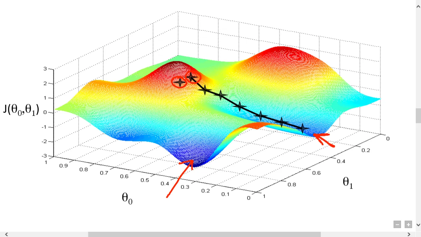
There is one more thing. Are you sure that you will always reach the same minimum? I can guarantee you are not sure. In case gradient descent you can’t be sure. Lets take the mountain problem. If you start few steps from your right It is entirely possible that you end up at completely different minima as shown in below image

Figure 12 : Problem with Gradient Descent(source : https://codesachin.wordpress.com/tag/gradient-descent/)

We will discuss the mathematical interpenetration of Gradient Descent but let’s understand some terms and notations as follows :

• alpha is learning rate which describes how big the step you take.
• Derivative gives you the slope of the line tangent to the ‘theta’ which can be either positive or negative and derivative tells us that we will increase or decrease the ‘theta’.
• Simultaneous update means that both theta should be updated simultaneously.

The derivation will be given by

Figure 13 : Gradient Descent Derivation

Normal Equations

As Gradient Descent is an iterative process, Normal equations help to find the optimum solution in one go. They use matrix multiplication. The formula’s and notations are explained in the images. Below right image will explain what will be our X and y from our example. The first column of our X will always be 1 because it will be multiplied by Theta_0 which we know is our intercept to the axis's.

Figure 14 : Normal Equation with Example

The derivation of the Normal Equation are explained in below image. They use matrix notation and properties.

This image explains the

• ‘Theta’ matrix
• ‘x’ matrix
• hypothesis is expanded
• Using those matrix we can rewrite the hypothesis as given is last step

Figure 15: Notations in Normal Equations

Figure 16 explains the following

• We will replace our hypothesis in error function.
• We assume z matrix as given in step 2
• Error Function can be rewritten as step 3. So if you multiply transpose of Z matrix with Z matrix. we will get our step 1 equation
• We can decompose z from step 2 as shown in step 4.
• By the property given in Step 6. We will rewrite z as given in Step 7. Capital X is also known as design matrix is transpose of small x

Figure 16 : Normal Equation Derivation Part 1

• Substituting z in the equation
• Expand the error equation and then take derivative with respect to theta and equate it to 0.
• We will get out solution. As shown in below image

Figure 17: Normal Equation Derivation Part 2

Comparison Between Gradient Descent and Normal Equations

• We need to choose alpha, initial value of theta in case of gradient Descent but Normal equations we don’t have to choose alpha or theta.
• Gradient Descent is an iterative process while Normal Equation gives you solution right away.
• Normal equation computation gets slow as number of features increases but Gradient Descent performs well with features being with very large.

We have seen linear regression is powerful algorithm for modeling relationship and predicting values based on that relationship. We have also discussed the methods of minimizing the error so that we can obtain the optimum values of our parameters. The linear Regression doesn’t perform well when it comes to classification problems. We will what algorithm overcomes that limitation in the next article. Keep Reading.

If you want to connect with me. Please feel free to connect with me on LinkedIn.

Sameer Negi — autonomous Vehicle Trainee — Infosys | LinkedIn