Learnt Harmonic Mean Estimator for Bayesian Model Selection
Machine learning assisted computation of the marginal likelihood
Bayesian model comparison provides a principled statistical framework for selecting an appropriate model to describe observational data, naturally trading off model complexity and goodness of fit. However, it requires computation of the Bayesian model evidence, also called the marginal likelihood, which is computationally challenging. We present the learnt harmonic mean estimator to compute the model evidence, which is agnostic to sampling strategy, affording it great flexibility.
This article was co-authored by Alessio Spurio Mancini.

Selection of an appropriate model to describe observed data is a critical task in many areas of data science, and science in general. The Bayesian formalism provides a robust and principled statistical framework for comparing and selecting models. However, performing Bayesian model selection is highly computationally demanding.
Bayesian model selection
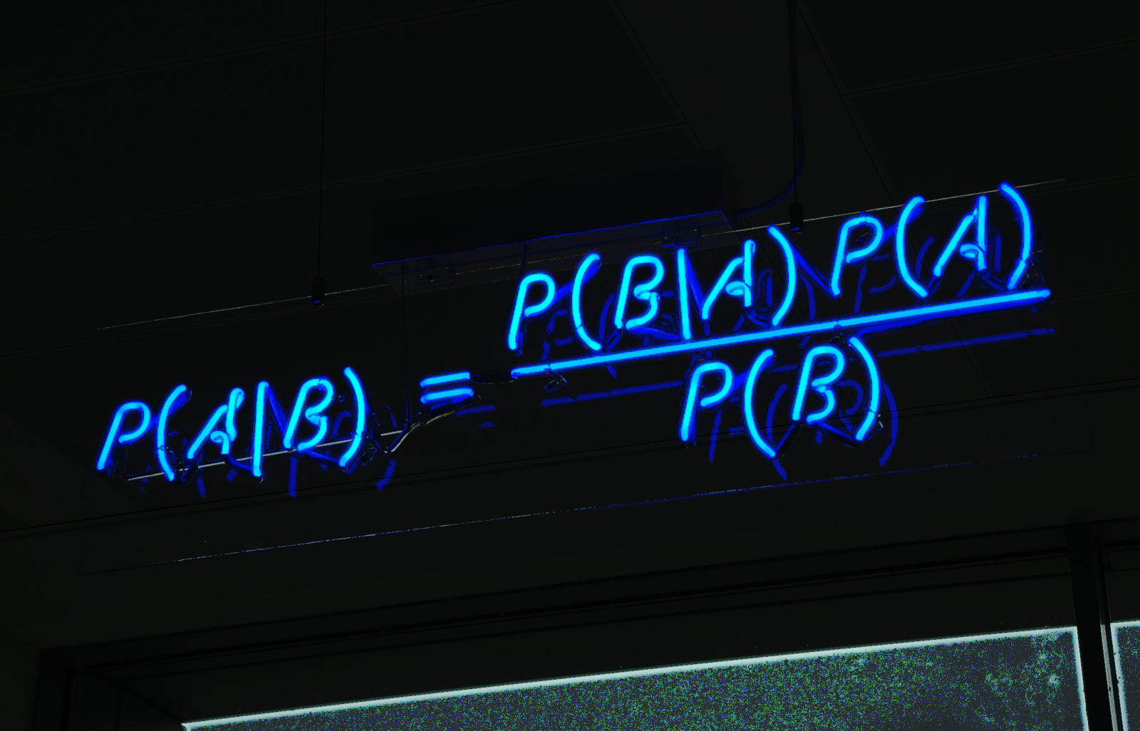
The Bayesian formalism is one of the most common approaches to statistical inference. For parameter inference, for a given model M, the posterior probability distribution of parameters of interest 𝜽 can be related to the likelihood of data y via Bayes’ theorem

where the prior distribution p(𝜽 | M) encodes our prior knowledge about the parameters before observation of the data (for an introduction to Bayesian inference see this excellent TDS article).
The Bayesian model evidence, given by the denominator of the equation above, is irrelevant for parameter estimation since it is independent of the parameters of interest and can simply be considered as a normalising constant. However, for model comparison the Bayesian model evidence, also called the marginal likelihood, plays a central role.
For model selection we are interested in the model posterior probability, which, by another application of Bayes’s theorem, can be written as

To compare models we therefore need to compute Bayes factors, which require computation of the model evidence of the models under consideration. This is where things get computationally challenging.
The Bayesian model evidence is given by the integral of the likelihood and prior over the parameter space:

Computation of the evidence therefore requires evaluation of a multi-dimensional integral, which can be highly computationally challenging. We will come back to this point shortly, introducing the learnt harmonic mean estimator to compute the model evidence.
It is insightful to note that the model evidence naturally incorporates Occam’s razor, trading off model complexity and goodness of fit, as illustrated in the following diagram.

The horizontal x-axis in the diagram above [1] represents all possible datasets. In the Bayesian formalism models are specified as probability distributions over datasets and, since probability distributions must sum to one, each model has a limited “probability budget” to allocate. While a complex model can represent a wide range of datasets well, it spreads its predictive probability widely. In doing so, the model evidence of complex models will be penalised if such complexity is not required.
The Bayesian formalism thus provides a principled statistical approach to perform model selection. Although, applying this formalism in practice is far from straightforward and is highly computationally challenging.
A variety of approaches to compute the model evidence have been developed, which have proven highly successful (e.g. [2,3,4,5]). These do, however, usually come with some restrictions and can be difficult to scale to higher dimensional settings. Computation of the model evidence is therefore far from a solved problem. In this article we focus on harmonic mean estimators to compute the Bayesian model evidence.
Original harmonic mean estimator
The original harmonic mean estimator was introduced in Newton & Raftery in 1994 [6] and relies on the following relationship:

This suggests the following estimator for the (reciprocal) of the model evidence:

The model evidence can thus be estimated from the harmonic mean of the likelihood, given samples from the posterior 𝜽ᵢ, which can be generated by Markov Chain Monte Carlo (MCMC) sampling.
A very nice property of the harmonic mean estimator is that is requires samples from the posterior only, which can be generated by any MCMC technique. In contrast, alternative approaches to compute the model evidence are typically tightly coupled to specific sampling approaches, which can be quite restrictive.
However, immediately after the harmonic mean estimator was proposed, it was realised that it can fail catastrophically [7]. In fact, the original harmonic mean estimator has been called the worst Monte Carlo method ever!
To gain intuition into why the original estimator can fail, it can be viewed from an importance sampling perspective. The estimator can be seen as importance sampling where the prior plays the role of the importance sampling target distribution and the posterior plays the role of the sampling density.
For importance sampling to be effective, we would typically consider a sampling density that is broader than the target. However, for the harmonic mean estimator we have the reverse since the prior distribution, which encapsulates our initial knowledge of the model parameters, is typically broader than the posterior, which encapsulates our knowledge of the model parameters after observation of the data. Consequently, the variance of the original harmonic mean can become very large and may not be finite, rendering the estimator ineffective in practice.
Re-targeted harmonic mean estimator
A re-targeted harmonic mean estimator was introduced by Gelfand & Dey in 1994 [8] to address this issue. The re-targeted harmonic mean estimator introduces a new target distribution φ(𝜽), which can be designed to avoid the problematic configuration discussed above, resulting in the following estimator:

The question remains: how should one select the new target distribution φ(𝜽)?
A variety of cases have been considered, for example a multivariate Gaussian [9] and indicator functions [10,11]. A Gaussian typically has tails that are too broad, acting to increase the variance of the estimator. While indicator functions have been shown to be effective [10], they often restrict to a small region of the parameter space and so can be inefficient.
Learnt harmonic mean estimator
One can gain further intuition into how to design an effective target distribution by considering the optimal target, which is nothing more than the normalised posterior itself (since the resulting estimator has zero variance). However, the target distribution must be normalised and the normalising constant of the posterior is the model evidence… precisely the term we are trying to estimate!
While the optimal target (the normalised posterior) is not accessible in practice, we propose estimating an approximation using machine learning:

This gives rise to the learnt harmonic mean estimator [12]. The learned approximation of the posterior need not be highly accurate. But, critically, it must not have fatter tails than the posterior. We impose this constraint when learning the target distribution from posterior samples. In addition, we propose strategies to estimate the variance of the learnt harmonic mean estimator, its own variance, and other sanity checks. (Further details can be found in our related article: McEwen et al. 2021 [12].)
Numerical experiments
We perform numerous numerical experiments to validate the learnt harmonic mean estimator by comparing to ground truth values of the Bayesian model evidence.
The Rosenbrock function provides a common benchmark for evaluating methods to compute the model evidence. In the following plot we show that the learnt harmonic mean estimator is robust and highly accurate for this problem.

Another common benchmark problem is the Normal-Gamma model, as illustrated graphically in the following diagram.

In a study reviewing estimators for computing the model evidence [13], this example was shown to present a pathological failure for the original harmonic mean estimator. In the table below we present the model evidence values computed for this problem by the original harmonic mean estimator and our learnt harmonic mean estimator. Our learnt estimator is highly accurate, providing an improvement over the original estimator by four orders of magnitude.

Harmonic code
The learnt harmonic mean estimator is implemented in the harmonic software package, which is open source and publicly available. Careful consideration has been given to the design and implementation of the code, following software engineering best practices.
Since the learnt harmonic mean estimator requires samples from the posterior distribution only, the harmonic code is agnostic to the method or code used to generate posterior samples. That said, harmonic works exceptionally well with MCMC sampling techniques that naturally provide samples from multiple chains by their ensemble nature, such as affine invariance ensemble samplers [14]. The emcee code [15] provides an excellent implementation of an affine invariance ensemble sampler and thus emcee is thus a natural choice for use with harmonic.
Summary
Bayesian model comparison provides a robust and principled statistical framework for selecting an appropriate model to describe observational data, naturally trading off model complexity and goodness of fit. However, it requires computation of the Bayesian model evidence, also called the marginal likelihood, which is a computationally challenging problem.
In this article we review harmonic mean estimators for computing the model evidence, including our recently proposed learnt harmonic mean estimator. The learnt harmonic mean estimator is agnostic to the method used to generate posterior samples, which affords it great flexibility. We have also released an open-source code, harmonic, that implements the estimator, where we have paid careful attention to the design and implementation of the code, following software engineering best practices.
At present, we adopt quite simple machine learning models with our learnt harmonic mean estimator. These simple models will struggle to scale to very high-dimensional settings. We are already exploring the use of more sophisticated machine learning models that will allow us to scale to yet higher dimensional settings.
We hope the learnt harmonic mean estimator can already provide a useful tool for Bayesian model selection. In particular, since it is agnostic to the sampling approach, it allows one to compute the model evidence for the large variety of sampling approaches where this has not been possible previously.
References
[1] Ghahramani, Bayesian non-parametrics and the probabilistic approach to modelling, Phil. Trans. R. Soc. A. (2013)
[2] Skilling, Nested sampling for general Bayesian computation. Bayesian Analysis (2006)
[3] Feroz & Hobson, MultiNest: an efficient and robust bayesian inference tool for cosmology and particle physics, MNRAS (2009), arXiv:0809.3437
[4] Handley, Hobson & Lasenby, PolyChord: nested sampling for cosmology, MNRAS (2015), arXiv:1502.01856
[5] Cai, McEwen, Pereyra, Proximal nested sampling for high-dimensional Bayesian model selection, arXiv:2106.03646
[6] Newton & Raftery, Approximate bayesian inference with the weighted likelihood bootstrap, J R Stat Soc Ser A (1994)
[7] Neal, Contribution to the discussion of “Approximate Bayesian inference with the weighted likelihood bootstrap” (1994)
[8] Gelfand & Dey, Bayesian model choice: asymptotics and exact calculations. J R Stat Soc Ser B (1994)
[9] Chib, Marginal likelihood from the Gibbs output, Journal of the American Statistical Association (1995)
[10] Robert & Wraith, Computational methods for Bayesian model choice, American Institute of Physics conference proceedings (2009),
arXiv:0907.5123
[11] van Haasteren, Marginal likelihood calculation with MCMC methods, In Gravitational Wave Detection and Data Analysis for Pulsar Timing Arrays (2014)
[12] McEwen, Wallis, Price, Docherty, Machine learning assisted Bayesian model comparison: learnt harmonic mean estimator (2021), arXiv:2111.12720
[13] Friel & Wyse, Estimating the evidence — a review, Statistica Neerlandica (2012), arXiv:1111.1957
[14] Goodman & Weare, Ensemble samplers with affine invariance, Communications in Applied Mathematics and Computational Science (2010)
[15] Foreman-Mackey, Hogg, Lang, Goodman, EMCEE: The MCMC hammer, PASP (2013), arXiv:1202.3665
