Learning to Rank: A Complete Guide to Ranking using Machine Learning

Published in

Towards Data Science

9 min readFeb 28, 2022

Ranking: What and Why?

In this post, by “ranking” we mean sorting documents by relevance to find contents of interest with respect to a query. This is a fundamental problem of Information Retrieval, but this task also arises in many other applications:

Search Engines — Given a user profile (location, age, sex, …) a textual query, sort web pages results by relevance.
Recommender Systems — Given a user profile and purchase history, sort the other items to find new potentially interesting products for the user.
Travel Agencies — Given a user profile and filters (check-in/check-out dates, number and age of travelers, …), sort available rooms by relevance.

Ranking applications: 1) search engines; 2) recommender systems; 3) travel agencies. (Image by author)

Ranking models typically work by predicting a relevance score s = f(x) for each input x = (q, d) where q is a query and d is a document. Once we have the relevance of each document, we can sort (i.e. rank) the documents according to those scores.

Ranking models rely on a scoring function. (Image by author)

The scoring model can be implemented using various approaches.

Vector Space Models – Compute a vector embedding (e.g. using Tf-Idf or BERT) for each query and document, and then compute the relevance score f(x) = f(q, d) as the cosine similarity between the vectors embeddings of q and d.
Learning to Rank – The scoring model is a Machine Learning model that learns to predict a score s given an input x = (q, d) during a training phase where some sort of ranking loss is minimized.

In this article we focus on the latter approach, and we show how to implement Machine Learning models for Learning to Rank.

Ranking Evaluation Metrics

Before analyzing various ML models for Learning to Rank, we need to define which metrics are used to evaluate ranking models. These metrics are computed on the predicted documents ranking, i.e. the k-th top retrieved document is the k-th document with highest predicted score s.

Mean Average Precision (MAP)

MAP — Mean Average Precision. (Image by author)

Mean Average Precision is used for tasks with binary relevance, i.e. when the true score y of a document d can be only 0 (non relevant) or 1 (relevant).

For a given query q and corresponding documents D = {d₁, …, dₙ}, we check how many of the top k retrieved documents are relevant (y=1) or not (y=0)., in order to compute precision Pₖ and recall Rₖ. For k = 1…n we get different Pₖ and Rₖ values that define the precision-recall curve: the area under this curve is the Average Precision (AP).

Finally, by computing the average of AP values for a set of m queries, we obtain the Mean Average Precision (MAP).

Discounted Cumulative Gain (DCG)

DCG — Discounted Cumulative Gain. (Image by author)

Discounted Cumulative Gain is used for tasks with graded relevance, i.e. when the true score y of a document d is a discrete value in a scale measuring the relevance w.r.t. a query q. A typical scale is 0 (bad), 1 (fair), 2 (good), 3 (excellent), 4 (perfect).

For a given query q and corresponding documents D = {d₁, …, dₙ}, we consider the the k-th top retrieved document. The gain Gₖ = 2^yₖ – 1 measures how useful is this document (we want documents with high relevance!), while the discount Dₖ = 1/log(k+1) penalizes documents that are retrieved with a lower rank (we want relevant documents in the top ranks!).

The sum of the discounted gain terms GₖDₖ for k = 1…n is the Discounted Cumulative Gain (DCG). To make sure that this score is bound between 0 and 1, we can divide the measured DCG by the ideal score IDCG obtained if we ranked documents by the true value yₖ. This gives us the Normalized Discounted Cumulative Gain (NDCG), where NDCG = DCG/IDCG.

Finally, as for MAP, we usually compute the average of DCG or NDCG values for a set of m queries to obtain a mean value.

Machine Learning Models for Learning to Rank

To build a Machine Learning model for ranking, we need to define inputs, outputs and loss function.

Input – For a query q we have n documents D = {d₁, …, dₙ} to be ranked by relevance. The elements xᵢ = (q, dᵢ) are the inputs to our model.
Output – For a query-document input xᵢ = (q, dᵢ), we assume there exists a true relevance score yᵢ. Our model outputs a predicted score sᵢ = f(xᵢ).

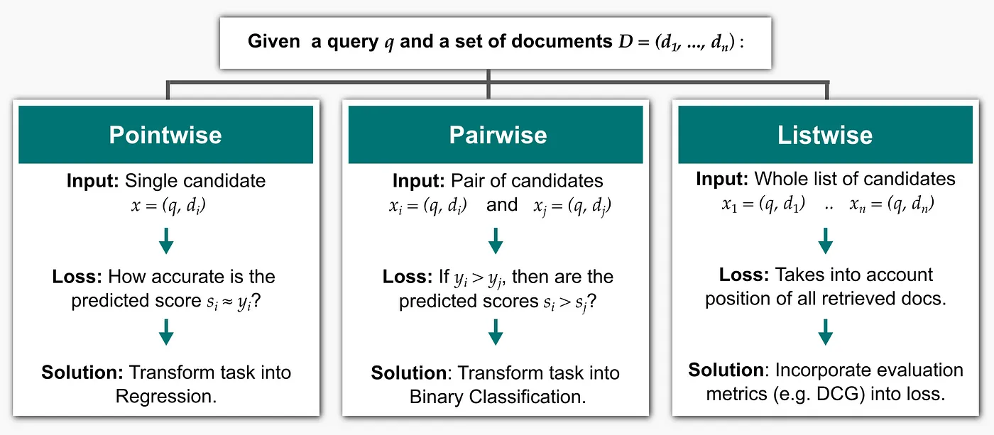
All Learning to Rank models use a base Machine Learning model (e.g. Decision Tree or Neural Network) to compute s = f(x). The choice of the loss function is the distinctive element for Learning to Rank models. In general, we have 3 approaches, depending on how the loss is computed.

Pointwise Methods – The total loss is computed as the sum of loss terms defined on each document dᵢ (hence pointwise) as the distance between the predicted score sᵢ and the ground truth yᵢ, for i=1…n. By doing this, we transform our task into a regression problem, where we train a model to predict y.
Pairwise Methods – The total loss is computed as the sum of loss terms defined on each pair of documents dᵢ, dⱼ (hence pairwise) , for i, j=1…n. The objective on which the model is trained is to predict whether yᵢ > yⱼ or not, i.e. which of two documents is more relevant. By doing this, we transform our task into a binary classification problem.
Listwise Methods – The loss is directly computed on the whole list of documents (hence listwise) with corresponding predicted ranks. In this way, ranking metrics can be more directly incorporated into the loss.

Machine Learning approaches to Learning to Rank: pointwise, pairwise, listwise. (Image by author)

Pointwise Methods

The pointwise approach is the simplest to implement, and it was the first one to be proposed for Learning to Rank tasks. The loss directly measures the distance between ground true score yᵢ and predicted sᵢ so we treat this task by effectively solving a regression problem. As an example, Subset Ranking uses a Mean Square Error (MSE) loss.

Pairwise Methods

The main issue with pointwise models is that true relevance scores are needed to train the model. But in many scenarios training data is available only with partial information, e.g. we only know which document in a list of documents was chosen by a user (and therefore is more relevant), but we don’t know exactly how relevant is any of these documents!

For this reason, pairwise methods don’t work with absolute relevance. Instead, they work with relative preference: given two documents, we want to predict if the first is more relevant than the second. This way we solve a binary classification task where we only need the ground truth yᵢⱼ (=1 if yᵢ > yⱼ, 0 otherwise) and we map from the model outputs to probabilities using a logistic function: sᵢⱼ = σ(sᵢ – sⱼ). This approach was first used by RankNet, which used a Binary Cross Entropy (BCE) loss.

BCE loss for pairwise methods as in RankNet. (Image by author)

RankNet is an improvement over pointwise methods, but all documents are still given the same importance during training, while we would want to give more importance to documents in higher ranks (as the DCG metric does with the discount terms).

Unfortunately, rank information is available only after sorting, and sorting is non differentiable. However, to run Gradient Descent optimization we don’t need a loss function, we only need its gradient! LambdaRank defines the gradients of an implicit loss function so that documents with high rank have much bigger gradients:

Gradients of an implicit loss function as in LambdaRank. (Image by author)

Having gradients is also enough to build a Gradient Boosting model. This is the idea that LambdaMART used, yielding even better results than with LambdaRank.

Listwise Methods

Pointwise and pairwise approaches transform the ranking problem into a surrogate regression or classification task. Listwise methods, in contrast, solve the problem more directly by maximizing the evaluation metric.

Intuitively, this approach should give the best results, as information about ranking is fully exploited and the NDCG is directly optimized. But the obvious problem with setting Loss = 1 – NDCG is that the rank information needed to compute the discounts Dₖ is only available after sorting documents based on predicted scores, and sorting is non-differentiable. How can we solve this?

A first approach is to use an iterative method where ranking metrics are used to re-weight instances at each iteration. This is the approach used by LambdaRank and LambdaMART, which are indeed between the pairwise and the listwise approach.

A second approach is to approximate the objective to make it differentiable, which is the idea behind SoftRank. Instead of predicting a deterministic score s = f(x), we predict a smoothened probabilistic score s~ 𝒩(f(x), σ²). The ranks k are non-continuous functions of predicted scores s, but thanks to the smoothening we can compute probability distributions for the ranks of each document. Finally, we optimize SoftNDCG, the expected NDCG over this rank distribution, which is a smooth function.

Uncertainty in scores produce a smooth loss in SoftRank. (Image by author)

A third approach is consider that each ranked list corresponds to a permutation, and define a loss over space of permutations. In ListNet, given a list of scores s we define the probability of any permutation using the Plackett-Luce model. Then, our loss is easily computed as the Binary Cross-Entropy distance between true and predicted probability distributions over the space of permutations.

Probability of various permutation using Plackett-Luce model in ListNet. (Image by author)

Finally, the LambdaLoss paper introduced a new perspective on this problem, and created a generalized framework to define new listwise loss functions and achieve state-of-the-art accuracy. The main idea is to frame the problem in a rigorous and general way, as a mixture model where the ranked list π is treated as a hidden variable. Then, the loss is defined as the negative log likelihood of such model.

LambdaLoss loss function. (Image by author)

The authors of the LambdaLoss framework proved two essential results.

All other listwise methods (RankNet, LambdaRank, SoftRank, ListNet, …) are special configurations of this general framework. Indeed, their losses are obtained by accurately choosing the likelihood p(y | s, π) and the ranked list distribution p(π | s).
This framework allows us to define metric-driven loss functions directly connected to the ranking metrics that we want to optimize. This allows to significantly improve the state-of-the-art on Learningt to Rank tasks.

Conclusions

Ranking problem are found everywhere, from information retrieval to recommender systems and travel booking. Evaluation metrics like MAP and NDCG take into account both rank and relevance of retrieved documents, and therefore are difficult to optimize directly.

Learning to Rank methods use Machine Learning models to predicting the relevance score of a document, and are divided into 3 classes: pointwise, pairwise, listwise. On most ranking problems, listwise methods like LambdaRank and the generalized framework LambdaLoss achieve state-of-the-art.

References

- Wikipedia page on “Learning to Rank”
- Li, Hang. “A short introduction to learning to rank.” 2011
- L. Tie-Yan. “Learning to Rank for Information Retrieval”, 2009
- L. Tie-Yan “Learning to Rank”, 2009
- X. Wang, “The LambdaLoss Framework for Ranking Metric Optimization”, 2018
- Z. Cao, “Learning to rank: from pairwise approach to listwise approach”, 2007
- M Taylor, “SoftRank: optimizing non-smooth rank metrics”, 2008