Interpreting CNN Models
How to get a good visual explanation of our predictions
TL;DR — Jump to Code
Grad-CAM gives you a class-discriminative visual explanation for the predictions of your CNN model. Guided Grad-CAM makes the visualization high resolution as well. You can find the code to generate the visualizations here.
The Problem
Nowadays machine learning models are being extensively used for automation and decision making. Model interpretability is crucial in both debugging these models as well as building trust in the system. When we use traditional machine learning solutions like tree-based models there is extensive tooling available for model interpretability. We can visualize the individual trees, plot partial dependence plots to understand the effect of different features on the target variable, use techniques like Shap values to compute feature importance or to explain the factors behind a single prediction, etc.
However, deep learning models are often treated as a black box. We throw in a lot of data, train a model, and hope it works. In this article, we will take a peek inside the black box of computer vision models — in particular, what is the model focusing on when making a prediction? Is it learning similar intuitions of humans and looking at the right things to make the right prediction?

What makes a good visual explanation?
For image classification, a ‘good’ visual explanation from the model for justifying any target category should satisfy two properties:
- Class Discriminative - It should be able to localize different regions in the input image which contributed to different output classes.
- High Resolution: It should be able to capture fine-grained detail.
Grad-CAM
Gradient-weighted Class Activation Mapping(Grad-CAM), uses the gradients of any target concept(say ‘dog’ in a classification network) flowing into the final convolutional layer to produce a coarse localization map highlighting the
important regions in the image for predicting the concept. Let’s break this down:
Why use the final convolutional layer?
Deeper layers in a CNN capture higher-level visual constructs. Furthermore, convolutional layers naturally retain spatial information which is lost in fully connected layers(often present in CNN architectures after the final convolutional layer), so we can expect the last convolutional layers to have the best compromise between high-level semantics and detailed spatial information. The neurons in these layers look for semantic class-specific information in the image(say object parts).
Generating a Class Activation Map
To generate the class activation map, we want to get the features detected in the last convolution layer and see which ones are most active when predicting the output probabilities. In other words, we can multiply each channel in the feature map array of the last convolutional layer by “how important this channel is” with regard to the output class and then sum all the channels to obtain a heatmap of relevant regions in the image.
CAM vs Grad-CAM
Traditional CAM uses the global average pooling weights to weigh the activations of the last convolutional layer. A drawback of CAM is that it requires feature maps to directly precede softmax layers, so it is only applicable to a particular kind of CNN architectures performing global average pooling over convolutional maps immediately prior to
prediction (i.e. conv feature maps → global average pooling
→ softmax prediction layer).
Grad-CAM uses the gradient information flowing into the last convolutional layer of the CNN to assign importance values. Grad-CAM is applicable to a
wide variety of CNN model-families
Seeing Grad-CAM in action
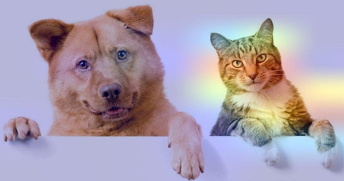
Let’s take an input image containing a cat and a dog and see how Grad-CAM fares.

Applying Grad-CAM results in a coarse heatmap of the same size as the convolutional feature maps

This heatmap can then be resized and superimposed on the original image. We can see that it is able to quite accurately identify the dog regions and the cat regions.

Application: Reducing Bias Using Grad-CAM
Let’s move away from cats and dogs and see a more practical usecase. Models trained on biased datasets may not generalize to real-world scenarios, or worse, may perpetuate biases and stereotypes (w.r.t. gender, race, age, etc.). Take an example of a model trained on image search results to identify nurses and doctors.
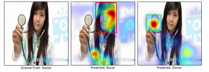
It turns out that the search results were gender-biased — 78% of images for doctors were men, and 93% of images for nurses were women. The biased model made the wrong prediction(misclassifying a doctor as a nurse) by looking at the face and the hairstyle. We use Grad-CAM to visualize the regions that the model is focusing on.
Using the intuitions gained from Grad-CAM visualizations, we reduced bias in the training set by adding in images of male nurses and female doctors, while maintaining the same number of images per class as before. The unbiased model made the right prediction looking at the white coat and the stethoscope. This is important not just for better generalization, but also for fair and ethical outcomes as more algorithmic decisions are made in
society
Going Further: High Resolution
Grad-CAM is able to produce class-discriminative visualisations. However, it generates a heatmap of the size of the final convoluational layer which is then resized to the size of the input image. Because of this, the heatmap is a coarse low resolution heatmap.
Guided Backpropogation
What if we take the gradients further to the input image instead of stopping at the final convoluational layer? It can produce a fine grained input pixel-level heatmap.
This backpropogation visualisation, often called saliency maps, can be generated by getting the gradient of the loss with respect to the image pixels. The changes in certain pixels that strongly affect the loss will be shown brightly. However, this often produces a noisy image and it has been shown that clipping the gradients less than zero during backpropogation(intuitively allowing only positive influences) gives a sharper image. This is similar to having a ReLU activation in forward propogation. The technique is called guided backpropogation.
Guided Backpropogation produces a heatmap of gradients of the same size as the input image. Since we do not need to resize a small feature map to the size of the input image, this is by-construction high resolution. However, the drawback here is that the visualisation is not class discriminative. You can see that both the dog and the cat parts of the image lights up corresponding to the loss of the dog.

Note, however that this visualization is still quite useful. This is just gradients in the size of the image but it clearly identifies a cat region, a dog region and a background region. This may be showing that if either the dog or the cat region changes(say the cat is shown more prominently or the dog is shown less prominently) — it can change the prediction.
Guided Grad-CAM
We can solve the fact that the Guided Backpropogation visualisation is not class discriminative by incorporating Grad-CAM heatmap as feature importances. This gives both a class-discriminative and a high resolution image.

Summary
Let’s not treat deep learning models as black boxes anymore. We need to develop more tools and techniques to peer inside the models and understand them. This is essential to verify that the models are not just making the right predictions but using the right signals to make them as well. Grad-CAM and Guided Grad-CAM provide an excellant way to understand the predictions of CNN models.
This is a colab notebook containing code to generate Grad-CAM, Guided Backpropogation and Guided Grad-CAM visualisations.
References
- Grad-CAM: Visual Explanations from Deep Networks via Gradient-based Localization, arXiv:1610.02391
- https://keras.io/examples/vision/grad_cam/
- https://github.com/ismailuddin/gradcam-tensorflow-2/blob/master/notebooks/GradCam.ipynb

