Insurance Risk Pricing — Tweedie Approach
An illustrative guide to estimate the pure premium using Tweedie models in GLMs and Machine Learning

Background
Insurance is a unique industry, probably one of the few where a company doesn’t know the actual cost of the product sold, they deal with the risks of unforeseeable events. Therefore, this industry has been relying on mathematics to understand the risk behavior of its customers and prospects for the last few centuries to estimate expected loss costs. Of course, methods have been evolving from Pascal’s triangle, application of probability, minimum bias procedures to generalized linear models and now machine learning.
Objective
We have discussed the count models (used in claim frequency) and the gamma model (used in claim severity) in previous articles in detail. The pure premium, also known as ‘loss cost’ is just the product of both the model estimates.
Claim Frequency = Claim Count / Exposure
Claim Severity = Claim Cost / Claim Count
Loss Cost = Claim Frequency x Claim Severity
In the current article, we are going to discuss a very important and interesting distribution called Tweedie, this distribution is interesting because it delivers many other distributions from Gaussian to inverse Gaussian by just changing a single parameter.
This distribution will help us in modeling pure premium directly without any need for two different models.
Tweedie Distribution
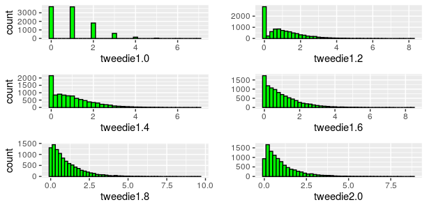
Tweedie distribution is a special case of exponential dispersion models and is often used as a distribution for generalized linear models. It can have a cluster of data items at zero and this particular property makes it useful for modeling claims in the insurance industry. This model can also be applied in other use cases across industries where you find a mixture of zeros and non-negative continuous data points.
If you see a histogram as below with a spike at zero, it’s a possible candidate to be fitted to a Tweedie model.

This family of distributions has the following characteristics
A mean, E(Y)= µ
A variance, Var(Y)= ϕµᵖ
Let’s understand with this expression “Y ~ Twₚ(µ,ϕ)”, where Y denote the response variable, Twₚ(µ,ϕ) denotes a Tweedie random variable with mean µ and variance ϕµᵖ and ϕ>0 and p ∈ (-∞,0 ] ∪[1,∞).
The p in the variance function is an additional shape parameter for the distribution.
An important point to be noted, this distribution is not defined for values of p between 0 and 1.
- If 1< p <2, the distribution are continuous for Y>0, with a positive mass at Y=0
- If p > 2, the distributions are continuous for Y > 0
Let’s look at Some of the commonly used members of the Tweedie family of distributions with their index parameter (p), variance function (V (µ)) and dispersion (ф)

One distribution enables fitting many other distributions. Setting p = 0 gives a normal distribution, p = 1 is Poisson, p = 2 gives a gamma distribution and p = 3 yields an inverse Gaussian.
Parameters conversion from one form to another.
We know Tweedie as a compound Poisson-Gamma distribution where a count N~Poisson(λ) and continuous number Z ~ Gamma(α,θ), in such case parameters can be easily translated into Tweedie parameters as given below:

Variance can also be translated — Var[Y] = ϕµᵖ =λ⋅θ² ⋅α (α+1)
Similarly, Tweedie parameters can also be converted into Poisson and Gamma parameters as follows:

Now, we got some understanding of this interesting distribution and its relation with its close family members like Poisson and Gamma.
Next, we will use a dataset and check this distribution’s applicability.
Recall our insurance dataset which we used in previous articles. We are hoping Tweedie distribution is the ideal candidate for this dataset, let’s explore this data to confirm our assumption.
This dataset (dataCar)can be downloaded from an R package called “insuranceData”.
library(insuranceData)
data(dataCar)
A brief overview of the dataset
This dataset is based on one-year vehicle insurance policies taken out in 2004 or 2005. There are 67,856 policies, of which 4624 (6.8% notified claims) filed claims.


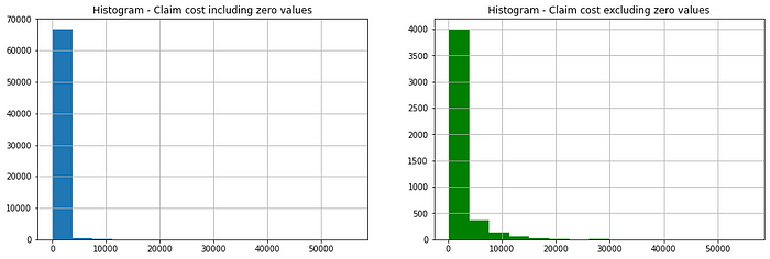
Only 7% of observation has positive values for the response variable, the rest of the values are zero. Let’s look at the distribution of claim count and cost independently.

As we have seen above
- Loss Cost = Claim Frequency x Claim Severity
Let’s re-write in terms of original variables
- Loss Cost = Claim Cost / Exposure
Response Variable — We are going to use ‘Claim Cost’ as a response variable keeping ‘exposure’ as an offset which is a suggested approach for modeling rates and averages.
Let’s have a look at the distribution of this variable.

We can see this data can not be fitted to the normal distribution, Poisson can also be discarded because this is not a count data. Another option we can think of Gamma, but this distribution does not take zero values. So, finally, we are left with Tweedie distribution which might be the best fit for this data.
Now, look at the independent variables. For detailed exploratory analysis and transformation of these variables, you can refer to the source code shared along with this article.
Independent Variables — We are going to use Vehicle body, vehicle age, driver’s age category, gender, area, and vehicle value as predictor variables. Claim occurrence indicator and the number of claims cannot be used as they are related to the dependent variable and can be known only after the event take place.
Derived Variable and Transformation — Vehicle body type by low frequencies can be grouped, also created an alternate categorical variable for vehicle value which can be tested for significance.
Selecting an optimal “p” for Tweedie model
Based on this exploratory analysis, we can confirm Tweedie distribution is an ideal candidate for fitting the model, but we are yet to find an optimum value for “p” which we know varies between 1 to 2.
Approach 1 — Manual selection of the variance power.
- Test a sequence of “p” between 1 to 2 by running iterative models.
- The Log-likelihood shows an inverse “U” shape.
- Select the “p” that corresponds to the “maximum” log-likelihood value.
- Fit the final model using that “p” value.
Approach 2 — Automated selection of variance power using statistical packages
Statistical packages (macros) are available in various software such as R, SAS, Python, and Emblem (Industry-specific software) to calculate maximum likelihood estimate for a series of “p” value. These are a kind of improvement to approach 1 with many other added features such as visualization. We can see the sample output below in the form of a graph generated from R using the “Tweedie” package.
#Maximum likelihood estimation of the Tweedie index parameter pest_p <-tweedie.profile(claimcst0 ~ veh_value+veh_body+veh_age+ gender+area+agecat,data=training,link.power = 0,do.smooth = TRUE, do.plot = TRUE)#Note
link.power - Index of power link function, link.power=0 produces a log-link
do.smooth - logical flag. If TRUE (the default), a spline is fitted to the data to smooth the profile likelihood plot. If FALSE, no smoothing is used (and the function is quicker)
do.plot - logical flag. If TRUE, a plot of the profile likelihood is produce. If FALSE (the default), no plot is produced

This graph shows that optimum “p” values lie somewhere between 1.5 and 1.6. We can use the suggested value for fitting the Tweedie model.
In Python, statsmodels has a function called estimate_tweedie_power for obtaining an optimum value.
Now, let’s train the model
We are using R and Python for fitting the Generalized Linear Models. R is quite mature in statistical models, python is also catching up with its statsmodels package. I feel a lack of proper examples and documentation for statsmodels is the only disadvantage.
In machine learning models, the Tweedie loss function is available in many algorithms such as GBM, LightGBM, XGBOOST, etc. Here, I will walk you through XGBOOST implementation.
Generalized Linear Models in R and Python
Implementation in R
library(tweedie)
library(statmod)#Model
tweedie_model <- glm(claimcst0 ~ veh_value+veh_body+veh_age+gender+ area+agecat,data=training, family = tweedie(var.power=1.6, link. power=0),offset=log(exposure))#Note
var.power -index of power variance function, for Tweedie it ranges between 1 to 2, here we are using 1.6.
link.power -index of power link function, link.power=0 produces a log-link
Implementation in Python, Statsmodels
import pandas as pd
import numpy as np
from patsy import dmatrices
import statsmodels.api as sm# Training and test splitmask = np.random.rand(len(df3)) < 0.8
df_train = df3[mask]
df_test = df3[~mask]
print('Training data set length='+str(len(df_train)))
print('Testing data set length='+str(len(df_test)))# Model expression
expr = """claimcst0 ~ veh_value_cat+veh_age+gender+area+agecat"""# Converting data into dmatrices
y_train, X_train = dmatrices(expr,df_train,return_type='dataframe')
y_test, X_test = dmatrices(expr, df_test, return_type='dataframe')# Training modeltweedie_model = sm.GLM(y_train, X_train,exposure=df_train.exposure, family=sm.families.Tweedie(link=None,var_power= 1.6,eql=True))tweedie_result = tweedie_model.fit()#Note
link - The default link for the Tweedie family is the log link. Available links are log and Power
var_power - The variance power. The default is 1
eql - If True, the Extended Quasi-Likelihood is used, else the likelihood is used (however the latter is not implemented). If eql is True, var_power must be between 1 and 2.
Model validation and goodness of fit in GLMs

We can analyze the results like any other regression, by looking at the results summary.
- If the p-value is less than or equal to the significance level, you can conclude that the variable is significant
- Other metrics such as AIC, Deviance, and Loglikelihood are useful for comparing related models. Lower the AIC and Deviance, better the model, whereas a higher value of the likelihood is better.
Implementation in Python, XGBOOST
import xgboost as xgb
from sklearn.metrics import mean_squared_error
from sklearn.model_selection import train_test_split#Segregating response and predictor variables in different data frameX, y = data.iloc[:,:-1],data.iloc[:,-1]
X_train, X_test, y_train, y_test = train_test_split (X,y,test_size =.2, random_state=123)#Creating DMatrix as required for this algorithmdtrain = xgb.DMatrix(data=X_train.iloc[:,1:28],label=y_train)
dtest = xgb.DMatrix(data=X_test.iloc[:,1:28],label=y_test)#Applying offsetdtrain.set_base_margin(np.log(X_train['exposure']))
dtest.set_base_margin(np.log(X_test['exposure']))#Setting Parametersparams =
{"objective":"reg:tweedie",'colsample_bytree': 1.0, 'learning_rate': 0.01,'gamma':1.5,'max_depth': 2, 'subsample':0.6, 'reg_alpha': 0,'reg_lambda':1,'min_child_weight':5, 'n_estimators':2000,
'tweedie_variance_power':1.6}xg_reg = xgb.train(params=params, dtrain=dtrain, num_boost_round=1000)#Note
reg:tweedie - Tweedie regression with log-link
tweedie_variance_power - default=1.5, range: (1,2)
Model validation in XGBOOST
Evaluation metrics like root mean squared error (rmse), mean absolute error (mae) and k-fold cross-validation techniques are some of the methods of validating and comparing the models.
preds = xg_reg.predict(dtest)
rmse = np.sqrt(mean_squared_error(y_test, preds))
print("RMSE: %f" % (rmse))
Please feel free to access complete code on my gist path.
Summary
We have discussed Tweedie distribution, one of the most commonly used distributions in the Insurance industry and its relation with other distributions of exponential dispersion models such as Poisson and Gamma. We also learned to estimate the Tweedie variance power which is the most important parameter required to fit an accurate model.
Though we discussed Tweedie implementation examples in some of the popular open-source packages, there are few more software that has this implementation which can be explored such as H2O, SAS, and Emblem.
Thanks for reading, hope you found the article informative. Please feel free to reach me for any queries or suggestions.
References
[1]Tweedie, M. C. K., “An Index which Distinguishes between Some Important Exponential Families,” in Statistics: Applications and New Directions, Proceedings of the Indian Statistical Golden Jubilee International Conference, J. K. Ghosh and J. Roy (Eds.), Indian Statistical Institute, 1984, 579–604


