Thoughts and Theory
Insights on the Calculus of Variations
Or how to prove that the shortest path between two points is a straight line
The calculus of variations is a powerful technique to solve some dynamic problems that are not intuitive to solve otherwise.
It is the precursor to optimal control theory as it allows us to solve non-complex control systems. Moreover, it is the basis for Lagrangian mechanics, less famous than its counterpart Newtonian mechanics yet just as powerful.
Understanding the calculus of variations framework will then allow you to put a steady foot in the optimal control theory framework as well as discovering key mathematical concepts.
Intuition on the theory
Contrary to function optimization theory, the calculus of variations does not try to find the minimum of a function. Instead, it enables us to find the ~minimum~ of a set of functions (which we call a functional). Each function is mapped to a single value by the mean of adding up a cumulative cost.
The problem we want to solve is finding a path, a set of continuous values, that leads to the minimum overall cost (any maximization problem can be turned into a minimization problem by adding a negative sign to the cost).
Take an investment company that can decide on its daily investments with a limited capital to use over one year. The money that is invested each day is generating a revenue on the same day. The company wants to earn as much possible over the year, and to do so sums up every day’s revenue into a yearly income. If the company has an investment simulation, it can try multiple investment strategies and determine what is the optimal sequence of daily investment through time (the path) that leads to the highest revenue. The simulation allows us to compare multiple investment paths and choose the one leading to the highest revenue.
Now why is the calculus of variations especially good at solving these problems?
Consider the case where we have to find the fastest transportation time riding metro. It is pretty easy to compare all possible combinations of metro stops and find out the optimal trajectory: in discretized space, the set of trajectories is a fixed number. Now consider the case where you are driving and need to rally point A to point B with full control on the steering wheel. The optimal trajectory does not depend on few metro line changes but on every single steering decision. In the continuous space, we are trying to compare an infinite number of possible trajectories, each of them varying infinitesimally from another one.
The calculus of variations provides a methodology to find out which path is the shortest in such a case.

The calculus of variation actually uses the same trick as function optimization. Function optimization would note that, at the optimal point, moving a little bit in any direction could only lead to a higher value, which would help to find out the first-order constraint on optimality.
The calculus of variations takes advantage of the fact that considering the optimal path, any path which differs a little bit from it would lead to a higher cost. From that observation, it is possible to derive the Euler-Lagrange equation which constitutes the base of the theory.
Solvable problems
We need to remind that the problems that can be solved by the calculus of variations are equivalent to minimizing the following expression:

Where y is our state variable, or the function for which you want to find the optimal path (i.e the daily investment), L your associated cost (i.e your daily revenue), and S the overall cost depending on which function y you chose (the yearly revenue).
Overall, the calculus of variations applies to the following type of problem:
- It is an optimization problem, which means it consists of minimizing (respectively maximizing) a certain value.
- The value to minimize is obtained by summing up a cost function from a given start to the end of the problem.
- The problem has a state variable for which we are trying to find an optimal set of values (the path).
- This cost function depends only on the state variable and its first-order derivative.
Let’s take a famous example often cited when presenting the calculus of variation theory: the shortest path.

The problem simply consists of demonstrating that the shortest path between two arbitrary points is a straight line. It looks obvious to us with our intuition-based brains, but the mathematical proof still requires the employment of the calculus of variations theory. Let’s check that this problem fits in:
- We are trying to minimize the length of a given path.
- The length of the path is the accumulation of segments lengths.
- The state variable is once again the geometrical path (coordinates of each segment).
- The length of a segment depends only on the orientation of each segment (the derivative of the state variable).
The problem that was considered in a preamble to optimal theory was the Brachistochrone, where we want to find the fastest trajectory leading a rolling bead to arrive at a given point.

Let’s check if each of these conditions applies:
- We are trying to minimize the duration of the rolling bead trajectory
- The trajectory duration is obtained by summing up the time that it takes the bead to go through successive segments of the trajectory
- The state variable is characterized by the coordinates of the successive segments of the trajectory (also known as a path).
- The time it takes for the bead to go through a segment of the trajectory depends only on the speed of the bead on a particular segment (that can be inferred from its height) and the length of the segment which again only depends on the derivative of the state variable.
To diversify, let’s take an example from economic sciences, which also relies on the calculus of variations: consider a factory that can manufacture a product given a rate of raw material income r(t) at a production rate p(r(t)).
The company faces multiple challenges:
- The earlier it gets money from the production the better
- Modifying the rate of production comes with a cost, increasing with the amount of change.
We can then represent this problem with the following equation:

Where the exponential term, usual in economics represents the decay of the value of the money earned (the loss of potential interests), U stands for unit price, C for unit cost, and K is a constant that affects how heavy the penalty is for increasing or decreasing the production rate too fast.
It’s pretty clear to see that we do have an overall value that we want to minimize (respectively maximize without the negative sign) being the overall revenue of the factory. The cumulated cost here is the revenue generated during a unit of time dt. Finally, the state variable, that we can freely choose and optimize, is the rate at which we decide to buy the income material at every time t. Finally, when looking at the equation, we realize that the cost function does only depends on t, r(t), r’(t) (since p is function of r). This problem, solvable using the calculus of variations technique, illustrates that some optimal control problems can be solved in a simple way using the method described in this article.
Now that we have seen multiple examples, we can try to reason on the type of problems that the calculus of variations enables us to deal with.
Obviously, if we look at the Brachistochrone and the factory problems, one word comes up to mind which is “dynamics” or in other terms, we are not only interested in the value of the state variable but how it evolves through time. This is clear by the fact that we do have the derivative of the state variable part of the equation. Not only we are concerned with the summation of a cost, but this cost is also sensitive to the rate of change of the state variable.
If you are being inquisitive, you would complain that the other example, the shortest path problem, does not look to have any dynamical aspect. This is actually not true. Instead consider the following problem: a car is moving forward at a fixed speed and can only modify its direction (which is the derivative of the given path). In this case, the cost to optimize is not the distance, but the time it took to rally the final destination.
Dynamical systems
What is to remember here is that the calculus of variations can help us solve some optimization problems for dynamical systems. But not every dynamical systems! Alas, only the first order ones.
As a reminder, a first order dynamical system is a system that can be fully described by a first order differential equation:

Take the shortest path problem (a.k.a constant speed car problem). The state variable of the problem, the position of the car, can be fully determined by first order differential equation. Now if you remind the problem used to introduce the optimal control theory, it was more or less the same problem:
A car is accelerating from given start and end positions with the objective of reducing the overall travel time, and the goal was to find out the optimal set of controls to apply on the gas pedal to reach the objective as fast as possible.
Both look like time optimal problems. The difference comes from the actual controls. The latter example allows to control the speed and acceleration of the car, thus position of the car cannot be determined by a first order differential equation.
Overall, we can say that the calculus of variations allows us to solve for paths, a drawn line, while it cannot solve for trajectories: a path with an idea of how fast we are moving through it.
Relationship with Lagrangian mechanics
In that sense, we can consider the calculus of variations as a tool to solve optimal control problems, but only for first-order dynamical systems.
In practice, most of systems are second-order dynamical systems. Think about physical systems evolving under Newton’s law of motion, its equation of motions depends on the acceleration of the system. If the acceleration is non-zero there is high chance that your system is a second-order dynamical system…
Unless it energy is constant. And this is all the trick about Lagrangian mechanics. Systems whose energy is constant are actually first-order systems. To make it clear, let’s write the following:

As can be seen, the system can be fully described without the acceleration appearing anywhere. This is a first-order dynamical system.
The brachistochrone is such a system, even though the acceleration of the bead is non-constant, as it is only evolving under the force of gravity and constraints on its position.
And that’s all what Lagrangian mechanics are about. Taking advantage of systems only under conservative forces (so that the total energy of the system is conserved), which makes them first-order dynamical systems thus eligible to be solved using Euler-Lagrangian equations.
We presented in the preamble to optimal control a general formulation for the Lagrangian equation of motion. Let’s detail it a bit here. Lagrange states and proves that finding the path characterizing the motion of a conservative system is equivalent to finding a stationary point of the following:

Here T represents the kinetic energy and V the potential energy of our system while y is a vector of coordinates of our choosing as long as it can fully represent the system in space at each time t. It could be cartesian coordinates as well as polar coordinates. The difference between the two entities has been stamped “Lagrangian”. If we can find the minimum of the integral of the Lagrangian over time, we then know that we found a stationary point and end up with a specific function of the system coordinates, the path.
The Lagrangian, difference between the kinetic and potential energy, seems a bit arbitrary. Why would minimizing such a cost result in finding the equations of motion for a system?
- First, because it works. If we use the Euler-Lagrange equations to solve for this specific problem where the Lagrangian is defined as the kinetic and potential energy difference, and if we choose Cartesian coordinates for the state variable, we end up with Newton’s laws of motions and it’s possible to derive in the other way as well.
- Second because it still makes some sense.
If you hold an object at a given height, this object has potential energy but no kinetic energy. If you drop it, you’ll observe that the potential energy is converted into kinetic energy. While we know that the total energy of the system is constant, this is not enough to know how the transition from potential to kinetic energy is performed and thus not enough to describe the laws of motion.
But we know that Nature is trying to minimize its energy spent, by keeping as much energy for itself as it can. When you blow a bubble, another kind of potential energy is involved linked to elastic deformation. The bubble lasts for a while as it tries to maintain its potential energy. You can assume the same for the object you are dropping. It is unwilling to move and will resist the force attracting it to the ground. We find that notion in Newtonian mechanics as the resistance to motion is called inertia. In that case, minimizing the kinetic energy while maximizing the potential energy is equivalent to minimizing (T — V).
The Lagrangian formulation can then be seen as trying to minimize the cost of motion.
Obviously, the Lagrangian formulation allows it to be solved using the calculus of variations framework: the Lagrangian only depends on the state variable r, its derivative r’ and time.
The biggest advantage that has Lagrangian mechanics over Newtonian mechanics is the possible use of any system of coordinates to describe the position of the system. This is very appreciable for any problem which involves rotational motions. This is due to the fact that the conservation of energy does not depend on any system of coordinates.
Lagrangian mechanics can be extended to adding constraints as long as they are holonomic (integrable). Basically, holonomic constraints are a set of equalities or inequalities that limit the path that you are trying to find. If you consider a 2D example as the shortest path problem, holonomic constraints would represent barriers that you place on the way to limit access to certain areas. These constraints in Newtonian mechanics are always forces acting on the system. For example for a pendulum, we express the tension of the link by a force for Newtonian mechanics, and by a constraint on the position of the pendulum for Lagrangian mechanics.
Last but not least, Lagrangian mechanics are limited to first-order dynamical systems. Any system including non-conservative forces (friction) needs to be solved using Newtonian mechanics.
Deriving the Euler-Lagrange equations
To find the equations of motion of a conservative system, Euler first came up with what is now called the Euler-Lagrange equations. They provide a first-order necessary condition to the problem. However, Lagrange revolutionized them by using the new notation epsilon, an infinitesimally small arbitrary number that changed the approach to the problem that Euler later called the calculus of variations. Let’s see how Lagrange did it.
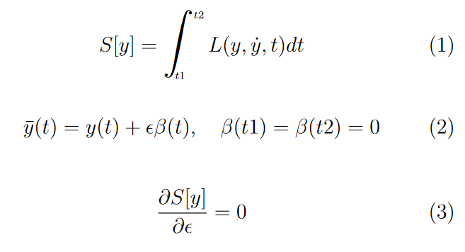
We first start with the definition of the problem:
(1) We want to find a stationary point of S[y]. For Lagrangian mechanics, the state corresponds to the space coordinates.
(2) is the trick: given the path of our system y(t), we consider the sets of paths that vary a little bit from that original path. We take a function beta which accounts for how much we vary at each point and epsilon which is an infinitesimally small value. We are analysing a small variation of a path, hence the calculus of variations. The only requirement over the path beta is that its start and end values are zero.
(3) is a direct translation of the definition of a stationary point. With the way we defined the new variable y bar, since beta is arbitrary, we actually have access to all possible paths. What we actually did is to introduce a new variable that enables us to browse through all solutions. In that sense, the functional S varies only with epsilon given this notation. Naturally, if we want to find a stationary point of S, then its first derivative needs to be zero with respect to epsilon.

(4) We are here deriving forward and applying the partial derivation chain rule. Notice that we are considering y bar in the derivation and not y as we are considering all possible variations of the original path y.
(5) By using equation (2), we can replace y bar in the partial derivatives with respect to epsilon with its actual expression.

(6) We are here applying the derivation by parts for the second term of the integral in equation (5). The goal is to get rid of the derivative of beta as we have no information about it. In the second term of equation (6), we see that we end up with [beta(t2)-beta(t1)]. Referring to (2), the extremities of the path beta are chosen to be 0, hence the second term is null.
(7) Simply rewriting the equation in a more compact shape having gotten rid of a term at the last step. We can state that this equality holds for any path beta (given the conditions in (2)). Since our equation is equal to 0 (3), the only way this is achievable is that at any time the term multiplying beta is null.
(8) Rewriting the result found in the last step with a minor difference. As you can see there are no more bars over the state variable y. This is due to the fact that we are evaluating the term for epsilon = 0 as the equation should hold for any epsilon. What we end up with are simply the Euler-Lagrange equations.
Note that what we did is a one-way derivation. That means the Euler-Lagrange equation provides a necessary condition but not a sufficient one.
Using the Euler-Lagrange equation
Armed with a powerful tool, we can try to solve the problems that we defined earlier.
- The brachistochrone
- The shortest path between two points
- Optimal factory production
- Equations of motions for conservative systems
The methodology to solve these problems is always the same.
1- We need to find an adequate state variable that can allow us to represent the system.
2- Express the Lagrangian (the cost) given the state variable.
3- Finally apply the Euler-Lagrangian to find a path that is a stationary point of the initial problem by transforming the problem formulation into a solvable one.
The shortest path problem
In the first place, let’s consider the shortest path problem and apply the three steps:
We consider two points A and B that we want to rally with the shortest path possible.
1- Since we are working in 2D, let’s choose cartesian coordinates. The state variable is then y(x), which constitutes a path.
2- Our total cost is the length of the path, which is characterized by the summation of the length of each segment, that we will define as dS. Using the Pythagoras theorem, we can also state that dS = sqrt(dx² + dy² ), which we can further factorize by dx. Note that dx/dy is simply y’.

Our functional does now look like this:

3- The Lagrangian is clearly identified here, and does only depend on y’. To use the Euler-Lagrange equation, we need to derive the Lagrangian with respect to y and y’.
The concept of derivating with respect to a derivated function can seem weird, but after all, in the first place, the state variable y is also a function. You need to remember that what we are considering from the start is a set of paths, where the state variable is a path itself. So as long as you consider that a path is a variable, then the derivative of the path is yet another variable.

We wrote the Euler-Lagrange equation with the state variable formulation that matches our problem and clearly defined the Lagrangian. The next step is simply to express the two terms of the Euler-Lagrange equation and derive to find out what is interesting to us: the expression of y*(x), the shortest path. Because in the end, that is exactly what the Euler-Equation is doing. It’s a necessary condition so that the path y minimizes T[y]. (Or at least is a stationary point of it).
As you can see, deriving with respect to y’ doesn’t pose any problem as long as we know that it is just a variable. By developing further, we reach a condition on y so that it does minimize T[y] and yields the shortest path:

A necessary condition on y to minimizes T[y] and to yield the shortest path is that y is a straight line, going from A to B.
The brachistochrone problem
The shortest path problem can be classified as rather simple to solve. Let’s see how we fare with a slightly more complex one, which was also the original problem that started the calculus of variations.
As a reminder, the system is a bead rolling frictionless from arbitrary point A to arbitrary point B. The bead is only under the force of gravity and the reaction of the bead.
The goal is to find the path that leads the bead to reach point B as fast as possible. Therefore it is a time-optimization problem.
1- There is necessarily a plane that contains point A and B. Let’s take the cartesian coordinates in that plane. The state variable is once again y(x).

2- Considering our cost, we want to minimize the time by which the bead reaches point B. We can say that it is the summation of the times that the bead needs to go over each segment of the path. But that does not relate very well to our state variable. Using the relation between time, distance, and speed we can say instead that our cost is the ratio dS/v where dS is the length of the segment and v(x, y) the velocity of the bead on the segment. Using Pythagoras theorem, we can use our state variable to express dS, to end up with the equivalent formulation:

However, we do not desire to have any additional dx in the formulation, since our state variable is y. We should there transform the equation so that only x, y or y’ are expressed. We first factorize the numerator so that dy/dx can be expressed as y’(x). On the denominator, we use to our advantage the law of energy conservation. When the bead of mass m is at A with altitude h, its energy is purely potential, therefore the energy of the system during the whole motion is constant and equal to mgh, and we can deduce from that the velocity of the bead for any given coordinates:

Step 2 is now complete, we have the expression of our cost, the Lagrangian, with respect to our state variable y and its derivate y’.
3- Let’s apply the Euler-Lagrange equations.
Since g and h are arbitrary, let’s focus on a case that simplifies our derivation: g= -1/2 and h=0. We get:

Since y is independent of y’, it is considered as a constant in the second equation. However, we do now need to derive with respect to x. And that’s when we have to remember that y’ and y do depend on x. By treating y as y(x) and y’ as y’(x), we can simply consider them as two independent functions each depending on x and perform the derivation. We find:

Putting together with the other part of the Euler-Lagrange equation, it is possible to perform some simplification (skipped here). We end up with:

To go from the first line to the second line, we multiply by y’. We then find out that it can be integrated, the result being the third line. (If you don’t believe me you can try to derive the last line again!).
At this point of the derivation, we have an equation that does look tractable. And by that, I mean that it can be easily solved by a numerical solver, while the initial formulation expressed as a functional is not solvable numerically. So that is what the Euler-Lagrange equation and the calculus of variations is about. Getting a necessary condition for the optimal path transforms the problem into a solvable one.
Now, for the brachistochrone, it is possible to fully solve the problem analytically. In the calculus of variations problems, we often end up with this kind of relationship between y and y’. The frequent solution to be able to identify the path y(x) is to take y’ as dy/dx, separate both dy and dx on each side of the equation, and integrate from start to end of the problem on each side. The rest of the derivation often includes making a smart change of variable. We know that for the brachistochrone problem the solution involves some curvy path. Hence a transformation from cartesian coordinates to angular variables seems to be a good move.
I will not detail the derivation here but know that it is possible to show that the optimal path that leads the shortest bead trajectory is a cycloid.

Calculus of variations with constraints
As we saw in a previous paragraph, to be able to solve dynamical systems using Lagrangian mechanics, we often need to use constraints and evoked the notion of Lagrangian multipliers.
If you are not familiar with Lagrange multipliers, the idea is basically to introduce a new variable, usually called lambda, that enables to transform a minimization problem into a system of equations using a specific relationship between the entity to minimize and the constraint, at the optimal point.
So if we consider this optimization problem:

We need a way to transform the system and make it into a formulation that is at least numerically solvable, if possible analytically solvable.
Lagrange observes that at the point where the minimum is reached given the constraint, the gradient of the surface f is pointing toward the same direction as the gradient of the constraint. This is due to the fact if you evolve through your surface looking at its contour lines (f(x) = constant), you’ll eventually reach a point where you only touch the constraint at a single point, hence the contour line is tangent to it. That means that gradients of both surfaces at this tangent point are collinear (but of opposite directions).

Since our input x is a vector of n components and we can have m constraint equations, the equation stated above will provide a system of n+m linear equations with n+m+1 variables. To make the system solvable, we still have to consider the initial constraint. Finding the minimum of f will then be equivalent to solving the following system:

Lambda (a scalar) is then considered as yet another variable in the system, and we can solve for it. We will eventually found a certain value of lambda, which doesn’t matter to us though.
That’s the theory for traditional function optimization. How would that translate to optimization of paths? The answer is, almost the same.
Lagrange states that, if we try to solve a problem of the form:
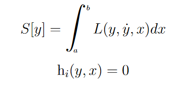
Then we can say that solving the above system is equivalent to solving:

In particular, we can express a new function, called the augmented Lagrangian L’ so that:

The way we introduce the lambda variable is similar to the function optimization problem. It is a bit harder to prove that the minimization problem stays equivalent with the two formulations, but the intuition is still the same.
Now instead of applying the Euler-Lagrange equation to the Lagrangian, we apply it to the augmented Lagrangian and proceed in the exact same way. You’ll end up with an extra variable to solve for, lambda, but this is the cost for making the problem actually solvable (analytically or numerically).
Limits to the Calculus of Variations
As we previously noted, second-order dynamical systems can not be solved using the Euler-Lagrange equation. Non-holonomic constraints also lead to the impossibility to solve the problem with this approach.
In particular, systems from control theory, for which we are not only trying to find the optimal path, but also the optimal set of controls for a given system to follow to that optimal path. Since we are controlling the system, which is most often a real-world physical system, controlling the system involves controlling its acceleration, hence making the equation not solvable with the Euler-Lagrange equation.
Another way to see it is that the expression of the controls for a system to optimize can be included in the optimization equation in the form of constraints:

Compared to the previous notation, the state variable y has been replaced by x, and the problem is time-dependent. Nonetheless, it should be obvious that the constraint includes the derivative of the state variable, making it non-holonomic.
Finally, we can analyse why such problems are not solvable with the calculus of variations through intuition. The theory is based on abstracting the group of all possible paths, and stating that any geometrical variation from that path would lead to a sub-optimized path. Since all variations are geometrical only, it is easy to translate this condition into the Euler-Lagrange equations by just taking one derivative. When we are applying a control over a system that can change its position, its speed, and its acceleration, varying from one path to another is not only geometrical, we also need to consider possible variations on the timing or variations on how fast a system is going to go through that new path. We can see that deriving a condition of optimality in such a scenario looks more difficult.
The problem was still solved analytically, dubbed the maximum principle, popularized by Lev Pontryagin. Pontryagin does find a condition for optimality with an approach similar to the one used for the calculus of variations, but of course much heavier mathematically.
In reality, however, optimal controls implemented for real applications do not rely much on the maximum principle. The tendency is more on approximating problems, for example by discretizing the state space and finding numerical approaches that try to reduce the need for heavy computation as much as possible. But understanding the calculus of variation theory is still beneficial to understand the field of control theory as a whole.
Sources:
[1] “Calculus of variations and optimal control theory, a concise introduction”, Daniel Liberzon.
[2] “ECON 402: Optimal Control Theory”, St. Francis Xavier University.
[3] “Physics 6010, Classical mechanics”, Utah State University.

