In the age of artificial intelligence, exact algorithms are not exactly hot. If a machine cannot learn it by itself, what’s the point? Why bother solving Markov Decision Process models with solutions that do not scale anyway? Why not dive straight into reinforcement learning algorithms?
It still pays off to learn the classical Dynamic Programming techniques. First of all, they are still widely used in practice. Many software developer jobs incorporate dynamic programming as part of their interview process. Although there are only so many states and actions you can enumerate, you may be surprised of the real-world problems that can still be resolved to optimality.
Second, even if only interested in reinforcement earning, many algorithms in that domain are firmly rooted in dynamic programming. Four policy classes may be distinguished in reinforcement learning, one of them being value function approximation. Before moving to such approaches, having an understanding of the classical value iteration algorithm is essential. Fortunately, it happens to be outlined in this very article.
Value iteration
The elegance of the value iteration algorithm is something to be admired. It really just takes a few lines of mathematical expressions, and not many more lines of code. Let’s check the seminal denotation by Sutton & Barto:
![Value iteration algorithm [source: Sutton & Barto (publicly available), 2019]](https://towardsdatascience.com/wp-content/uploads/2021/12/1Rg3xj63Uwbw7_pBgEqEJdA.png)
The intuition is fairly straightforward. First, you initialize a value for each state, for instance at 0.
Then, for every state you compute the value V(s), by multiplying the reward for each action a (direct reward r+ downstream value V(s')) with the transition probability p.
Suppose we indeed initialized at 0 and direct rewards r are non-zero. The discrepancies will directly become visible in the difference expression |v-V(s)|, where v is the old estimate and V(s) the new one. So, the error Δ will exceed the threshold θ (a small value) and a new iteration follows.
By performing sufficiently many iterations, the algorithm will converge to a point where |v-V(s)|<θ for every state. You can then resolve the argmax to find the optimal action for each state; knowing the true value functions V(s) equates having the optimal policy π.
Note that optimality is not guaranteed ifθ is set too large. For practical purposes a reasonably small error tolerance will do, but for the mathematical sticklers among us it is good to keep in mind the optimality conditions.
A minimal working example
With the mathematics out of the way, let’s continue with the coding example. To keep the focus on the algorithm, the problem is extremely simple.
The problem
Consider a one-dimensional world (a row of tiles), with a single terminating state. Hitting the terminating state yields a reward of +10, every other action costs -1. The agent can move left or right, but – to not make it too trivial -the agent moves into the wrong direction 10% of the time. It’s a very simple problem, but it has (i) a direct reward, (ii) an expected downstream reward, and (iii) transition probabilities.
The algorithm
The Python algorithm stays pretty close to the mathematical outline provided by Sutton & Barto, so no need to expand too much. The full code fits in a single Gist:
Some experiments
Ok, some experiments then. We start by showing two iterations of the algorithm in full detail.
First, we set v equal to V(0), which is 0:v=V(0)=0
Next, we update V(0). Note r is fixed for each state; we effectively only sum over the set of next states via s'.
![Value iteration step 1, state 0 [image by author]](https://towardsdatascience.com/wp-content/uploads/2021/12/14No0QEdh1J0v06FqKqz-pA.png)
That seems like a lot of computational effort for such a small problem. Indeed, it’s easy to see why dynamic programming does not scale well. In this case, all values V(s) are still at 0 – as we just started – so the estimated state value V(0) is simply the direct reward -1.
Let’s try one more, somewhat further along the line. Same computation, but now the values V(s) have been updated throughout several iterations. We now have V=[5.17859, 7.52759, 10.0, 7.52759, 5.17859]. Again, we plug in the values:
![Value iteration step 4, state 0 [image by author]](https://towardsdatascience.com/wp-content/uploads/2021/12/1JYX5aS6CA6sOVXlFBY3-cg.png)
Thus, we update V(0) from 5.18 to 5.56. The error would be Δ=(5.56–5.18)=0.38. In turn, this will affect the updates of the other states, and this process continues until Δ<θ for all states. For state 0, the optimal value is 5.68, hit within 10 iterations.
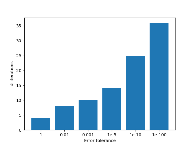
The most interesting parameter to test here is the error tolerance θ, which influences the numbers of iterations before convergence.
Final words
Value iteration is one of the cornerstones for Reinforcement Learning. It is easy to implement and understand. Before moving towards more advanced implementations, make sure to grasp this fundamental algorithm.
Some other minimal working examples you might be interested in:
Implement Policy Iteration in Python – A Minimal Working Example
A Minimal Working Example for Deep Q-Learning in TensorFlow 2.0
A Minimal Working Example for Continuous Policy Gradients in TensorFlow 2.0
A Minimal Working Example for Discrete Policy Gradients in TensorFlow 2.0
References
Sutton, Richard S., and Andrew G. Barto. Reinforcement learning: An introduction. MIT press, 2018.