Image Processing with Python — Unsupervised Learning for Image Segmentation
How to use the K-Means algorithm to automatically segment an image

So far most of the techniques we’ve gone over have required us to manually segment the image via its features. But we can actually use unsupervised clustering algorithms to do this for us. In this article we shall go over how to do just that.
Let’s begin!
As always, we start by importing the required Python libraries.
import numpy as np
import pandas as pd
import matplotlib.pyplot as pltfrom mpl_toolkits.mplot3d import Axes3D
from matplotlib import colors
from skimage.color import rgb2gray, rgb2hsv, hsv2rgb
from skimage.io import imread, imshow
from sklearn.cluster import KMeans
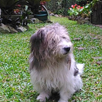
Excellent, let us now import the image we will be working with.
dog = imread('beach_doggo.PNG')
plt.figure(num=None, figsize=(8, 6), dpi=80)
imshow(dog);
We know that an image is essentially a 3 Dimensional matrix, with each individual pixel containing a value for the Red, Green, and Blue channels. But we can actually use the beloved Pandas library to store each pixel as a separate data point. The below code does just that.
def image_to_pandas(image):
    df = pd.DataFrame([image[:,:,0].flatten(),
                       image[:,:,1].flatten(),
                       image[:,:,2].flatten()]).T
    df.columns = [‘Red_Channel’,’Green_Channel’,’Blue_Channel’]
    return dfdf_doggo = image_to_pandas(dog)
df_doggo.head(5)

This makes the manipulation of the image simpler as it is easier to think of it as data that can be fed into a machine learning algorithm. In our case we shall make use of the K Means algorithm to cluster the image.
plt.figure(num=None, figsize=(8, 6), dpi=80)
kmeans = KMeans(n_clusters=  4, random_state = 42).fit(df_doggo)
result = kmeans.labels_.reshape(dog.shape[0],dog.shape[1])
imshow(result, cmap='viridis')
plt.show()
As we can see, the image is clustered into 4 distinct regions. Let us visualize each region separately.
fig, axes = plt.subplots(2,2, figsize=(12, 12))
for n, ax in enumerate(axes.flatten()):
    ax.imshow(result==[n], cmap='gray');
    ax.set_axis_off()

fig.tight_layout()
As we can see, the algorithm splits the the image based on the R,G, and B pixel values. One unfortunate drawback of course is that this is a completely unsupervised learning algorithm. It does not particularly care for the meaning behind any specific cluster. As evidence we can see that the second and fourth cluster both have a prominent part of the dog (the shaded half and the unshaded half). Perhaps running 4 clusters is excessive, let us retry the clustering but set the number of clusters to 3.

Excellent, we can see that the dog comes out as a whole unit. Now let us see what happens if we apply each cluster as a separate mask to our image.
fig, axes = plt.subplots(1,3, figsize=(15, 12))
for n, ax in enumerate(axes.flatten()):
    dog = imread('beach_doggo.png')
    dog[:, :, 0] = dog[:, :, 0]*(result==[n])
    dog[:, :, 1] = dog[:, :, 1]*(result==[n])
    dog[:, :, 2] = dog[:, :, 2]*(result==[n])
    ax.imshow(dog);
    ax.set_axis_off()
fig.tight_layout()
We can see that the algorithm generates three distinct clusters, the sand, the living creatures, and the sky. Of course the algorithm itself does not care much for these clusters, only that they share similar RGB values. It is up to us humans to interpret these clusters.
Before we leave, I think it would be helpful to actually show what our image looks like if we simply plotted it out on a 3D graph.
def pixel_plotter(df):
    x_3d = df['Red_Channel']
    y_3d = df['Green_Channel']
    z_3d = df['Blue_Channel']

    color_list = list(zip(df['Red_Channel'].to_list(),
                          df['Blue_Channel'].to_list(),
                          df['Green_Channel'].to_list()))    norm = colors.Normalize(vmin=0,vmax=1.)
    norm.autoscale(color_list)
    p_color = norm(color_list).tolist()

    fig = plt.figure(figsize=(12,10))
    ax_3d = plt.axes(projection='3d')
    ax_3d.scatter3D(xs = x_3d, ys =  y_3d, zs = z_3d,
                    c = p_color, alpha = 0.55);

    ax_3d.set_xlim3d(0, x_3d.max())
    ax_3d.set_ylim3d(0, y_3d.max())
    ax_3d.set_zlim3d(0, z_3d.max())
    ax_3d.invert_zaxis()


    ax_3d.view_init(-165, 60)pixel_plotter(df_doggo)

We should bear in mind that this is actually how the algorithm defines “closeness”. If we apply the K-Means algorithm to this graph, the manner by which it segments the image becomes strikingly clear.
df_doggo['cluster'] = result.flatten()def pixel_plotter_clusters(df):
    x_3d = df['Red_Channel']
    y_3d = df['Green_Channel']
    z_3d = df['Blue_Channel']

    fig = plt.figure(figsize=(12,10))
    ax_3d = plt.axes(projection='3d')
    ax_3d.scatter3D(xs = x_3d, ys =  y_3d, zs = z_3d,
                    c = df['cluster'], alpha = 0.55);

    ax_3d.set_xlim3d(0, x_3d.max())
    ax_3d.set_ylim3d(0, y_3d.max())
    ax_3d.set_zlim3d(0, z_3d.max())
    ax_3d.invert_zaxis()


    ax_3d.view_init(-165, 60)pixel_plotter_clusters(df_doggo)

In Conclusion
The K-Means algorithm is a popular unsupervised learning algorithm that any data scientist should be comfortable using. Though it is quite simplistic, it can be particularly powerful on images that have very distinct differences in their pixels. In future articles we shall go over other machine learning algorithms we can use for image segmentation as well as fine tuning the hyper parameters. But for now I hope you can now imagine using this method on your own tasks.