Image Processing for Python — Adjusting to the Ground Truth
Ground Truth Algorithm for Beginners

In this lesson we shall go over an image adjustment algorithm which may be intuitive for most readers. Unlike the other image adjustment algorithms we have discussed so far (such as RGB Channel Adjustment and Histogram Manipulation), this method will use the actual colors available in the image.
Let’s get started!
As always, we must import the required Python Libraries.
import numpy as np
import matplotlib.pyplot as plt
from matplotlib.patches import Rectangle
from skimage.io import imread, imshow
import skimage.io as skio
from skimage import img_as_ubyte, img_as_float
Great, now let us look at the image we’re working with.
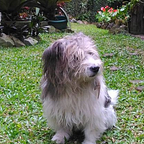
overcast = imread("image_overcast.PNG")
plt.figure(num=None, figsize=(8, 6), dpi=80)
imshow(overcast);
The image clearly has a color overcast. Now let us try to adjust it.
To begin we must first select the particular ground truth patches we want the machine to work with. To do that we can use the Rectangle function available in NumPy.
fig, ax = plt.subplots(1,1, figsize=(8, 6), dpi = 80)
patch = Rectangle((70,175), 10, 10, edgecolor='r', facecolor='none')
ax.add_patch(patch)
ax.imshow(overcast);
We can see the red rectangle on the upper left corner of the image. I’m sure most of you suspect that this may not be the best ground truth patch to use. The reason being that it is quite different from the rest of the image. However, for pedagogical reasons we shall use this square and adjust our image to it.
Let us first get a close up view of our ground truth patch. To do that we must use the get_bbox() and get_points() functions found in NumPy.
coord = Rectangle.get_bbox(patch).get_points()
print(coord)
We can now use this coordinate array to slice our main image.
fig, ax = plt.subplots(1,1, figsize=(8, 6), dpi = 80)
ax.imshow(overcast[int(coord[0][1]):int(coord[1][1]),
                   int(coord[0][0]):int(coord[1][0])]);
As we can see, the ground truth patch is far from a monotonic color. Within it are multiple shades of brown and black (a testament to the amount of details not visible to the human eye!).
Now let us actually adjust our image to the patch. We shall use the Max and Mean values of the patch.
image_patch = overcast[int(coord[0][1]):int(coord[1][1]),
                       int(coord[0][0]):int(coord[1][0])]image_max = (overcast / image_patch.max(axis=(0, 1))).clip(0, 1)
image_mean = ((overcast * image_patch.mean())
               / overcast.mean(axis=(0, 1))).clip(0,255).astype(int)
fig, ax = plt.subplots(1,2, figsize=(15, 10), dpi = 80)
f_size = 19
ax[0].imshow(image_max)
ax[0].set_title('Max Adjusted', fontsize = f_size)
ax[0].set_axis_off()ax[1].set_title('Mean Adjusted', fontsize = f_size)
ax[1].imshow(image_mean);
ax[1].set_axis_off()
fig.tight_layout()

As we can see, both adjustments are pretty terrible. Depending on your preference you could say either is better. The Max adjusted image (though clearly overexposed) does highlight the green color of the plant on the left as well as the blue cap of the carriage driver on the right. The Mean adjusted image (though extremely faded) does fair better in terms of overall clarity of the image. But I believe it is safe to say that neither of these adjustments would do. To remedy this let us go back to the selection of ground truth patches.
fig, ax = plt.subplots(1,1, figsize=(8, 6), dpi = 80)
patch1 = Rectangle((100,300), 10, 10, edgecolor='r',
                    facecolor='none')
patch2 = Rectangle((200,250), 10, 10, edgecolor='r',
                    facecolor='none')
patch3 = Rectangle((200,190), 10, 10, edgecolor='r',
                    facecolor='none')ax.add_patch(patch1)
ax.add_patch(patch2)
ax.add_patch(patch3)
ax.imshow(overcast);

Though we do not have to, we can plot out the patches so that we can get an idea of what they look like.
coor1 = Rectangle.get_bbox(patch1).get_points()
coor2 = Rectangle.get_bbox(patch2).get_points()
coor3 = Rectangle.get_bbox(patch3).get_points()image_patch1 = overcast[int(coor1[0][1]):int(coor1[1][1]),
                        int(coor1[0][0]):int(coor1[1][0])]image_patch2 = overcast[int(coor2[0][1]):int(coor2[1][1]),
                        int(coor2[0][0]):int(coor2[1][0])]image_patch3 = overcast[int(coor3[0][1]):int(coor3[1][1]),
                        int(coor3[0][0]):int(coor3[1][0])]fig, ax = plt.subplots(1,3, figsize=(15, 12), dpi = 80)
ax[0].imshow(image_patch1)
ax[1].imshow(image_patch2)
ax[2].imshow(image_patch3);

Like our first patch, these patches also show an array of colors. Let us now use each one in adjusting our image. To aid in this, let us first use Python’s list comprehension capabilities to create a list of the adjusted images.
patch_list = [image_patch1, image_patch2, image_patch3]
image_max_list = [(overcast / patch.max(axis=(0, 1))).clip(0, 1) for
                   patch in patch_list]
image_mean_list = [((overcast * patch.mean()) / overcast.mean(axis=(0, 1))).clip(0, 255).astype(int) for
                   patch in patch_list]
Wonderful! Now we can simply call all these images.
Let us begin.
def patch_plotter(max_patch, mean_patch):
    fig, ax = plt.subplots(1,2, figsize=(15, 10), dpi = 80)
    f_size = 19
    ax[0].imshow(max_patch)
    ax[0].set_title('Max Adjusted Patch', fontsize = f_size)
    ax[0].set_axis_off()    ax[1].set_title('Mean Adjusted Patch', fontsize = f_size)
    ax[1].imshow(mean_patch);
    ax[1].set_axis_off()
    fig.tight_layout()for i in range(3):
    patch_plotter(image_max_list[i], image_mean_list[i])


We can see from the results that the Max adjusted patches perform much better than the Mean adjusted patches. Furthermore, it seems that the second patch faired the best. This seems to indicate that best batch is one that adjusts the image to a beige-like color. As a final exercise let us choose patches that fit that particular description. Also, we shall decrease the size of the patches to lessen the amount of color variety in the patches.
Below is a function that can generate the ground truth adjusted images. We simply need to feed it our image, the names of the patches (for labelling purposes), and the patch coordinates.
def ground_truth(image, patch_names, patch_coordinates):
    f_size = 25
    figure_size = (17,12)
    patch_dict = dict(zip(patch_names, patch_coordinates))
    coord = []

    fig1, ax_1 = plt.subplots(1, 3, figsize = figure_size)
    for n, ax in enumerate(ax_1.flatten()):
        #Create Rectangles
        key = list(patch_dict.keys())[n]
        patch = Rectangle(patch_dict[key], 5, 5, edgecolor='r',
        facecolor='none')
        coord.append(Rectangle.get_bbox(patch).get_points())
        ax.add_patch(patch);

        #Show and Format Images
        ax.imshow(image)
        ax.set_title(f'{key}', fontsize = f_size)
        ax.set_axis_off()
    fig1.tight_layout()

    fig2, ax_2 = plt.subplots(1, 3, figsize = figure_size)

    for n, ax in enumerate(ax_2.flatten()):
        #Show and Format Rectangles
        key = list(patch_dict.keys())[n]
        ax.imshow(image[int(coord[n][0][1]) : int(coord[n][1][1]),
                        int(coord[n][0][0]) : int(coord[n][1][0])]);
        ax.set_title(key, fontsize = f_size)
        ax.set_axis_off()

    fig2.tight_layout()fig3, ax_3 = plt.subplots(1, 3, figsize = figure_size)
    for n, ax in enumerate(ax_3.flatten()):
        patch =image[int(coord[n][0][1]) : int(coord[n][1][1]),
                     int(coord[n][0][0]) : int(coord[n][1][0])]

        image_max = (image / patch.max(axis=(0, 1))).clip(0, 1)
        ax.imshow(image_max)
        ax.set_title(f'Max : {patch_names[n]}', fontsize = f_size)
        ax.set_axis_off()fig3.tight_layout()ground_truth(overcast,
             ['First', 'Second', ' Third'],
             [(105, 275), (50, 45), (330, 105)])

We can see that among the different ground truth patches, the third patch performs the best. Though the image is noticeable bluer, the yellow overcast was completely removed. Additionally, overexposure is kept at a bare minimum.
In Conclusion
We see that one does not need to be extremely well versed in the different ways color is interpreted by the machine. We can use the simple yet effective Ground Truth algorithm to adjust our images. This particular method may be more suited for individuals with an intuitive understanding of colors. Though good results did take a while to achieve, this method is worth keeping in mind as it one of the more straightforward ways to alter an image.
I hope that you have learned the significance of this more simple algorithm.